Wolfram Language Paclet Repository

Community-contributed installable additions to the Wolfram Language

Primary Navigation

    • Cloud & Deployment
    • Core Language & Structure
    • Data Manipulation & Analysis
    • Engineering Data & Computation
    • External Interfaces & Connections
    • Financial Data & Computation
    • Geographic Data & Computation
    • Geometry
    • Graphs & Networks
    • Higher Mathematical Computation
    • Images
    • Knowledge Representation & Natural Language
    • Machine Learning
    • Notebook Documents & Presentation
    • Scientific and Medical Data & Computation
    • Social, Cultural & Linguistic Data
    • Strings & Text
    • Symbolic & Numeric Computation
    • System Operation & Setup
    • Time-Related Computation
    • User Interface Construction
    • Visualization & Graphics
    • Random Paclet
    • Alphabetical List
  • Using Paclets
    • Get Started
    • Download Definition Notebook
  • Learn More about Wolfram Language

QuantumFramework

Tutorials

  • Bell's Theorem: CHSH inequality
  • Circuit Diagram
  • Exploring Fundamentals of Quantum Theory
  • Getting Started
  • An IBM Quantum Error Map
  • Connecting to QPU Services
  • Quantum Machine Learning in Phase Space
  • Quantum object abstraction
  • Quantum Object Composition
  • Quantum Optimization
  • Second Quantization Functions
  • Sending Queries to IBM QPUs
  • Tensor Network
  • Time Evolution
  • Fast Gates on a Transmon
  • Quantum Computation

Guides

  • Wolfram Quantum Computation Framework

Symbols

  • CliffordChannel
  • EinsteinSummation
  • GraphState
  • IBMJob
  • IBMJobSubmit
  • LocalComplement
  • PauliStabilizer
  • QiskitCircuit
  • QiskitTarget
  • QuantumBasis
  • QuantumChannel
  • QuantumCircuitMultiwayGraph [EXPERIMENTAL]
  • QuantumCircuitOperator
  • QuantumDistance
  • QuantumEntangledQ
  • QuantumEntanglementMonotone
  • QuantumEvolve
  • QuantumMeasurement
  • QuantumMeasurementOperator
  • QuantumMeasurementSimulation
  • QuantumMPS [EXPERIMENTAL]
  • QuantumOperator
  • QuantumPartialTrace
  • QuantumPhaseSpaceTransform
  • QuantumQASM
  • QuantumShortcut [EXPERIMENTAL]
  • QuantumSimilarity
  • QuantumStateEstimate [EXPERIMENTAL]
  • QuantumState
  • QuantumTensorProduct
  • QuantumWignerMICTransform [EXPERIMENTAL]
  • QuantumWignerTransform [EXPERIMENTAL]
  • QuditBasis
  • QuditName
  • StabilizerFrame
  • StabilizerStateQ

Fast Gates on a Transmon

Five Levels of a Transmon
DRAG
The Pulse
Decoherence and the Best Pulse Length
Leakage
Five Levels Are Enough
A transmon is a superconducting circuit that behaves as a weakly anharmonic oscillator. A qubit is stored in its two lowest levels, and a microwave pulse at the qubit frequency rotates it between them. The anharmonicity is small, a few hundred megahertz against a qubit frequency of several gigahertz, so the transition from |1⟩ to |2⟩ lies close to the qubit transition. A short pulse has a broad spectrum and drives both, carrying population out of the qubit. A long pulse avoids that but is exposed for longer to energy decay and dephasing.
How long the best pulse is, and how much the derivative correction known as DRAG shortens it, has no closed-form answer. Both follow from the Schrödinger and Lindblad equations solved with the levels the qubit leaks into kept explicitly. For an anharmonicity of −200 MHz and coherence times
T
1
and
T
2
of 100 μs, the best π pulse below lasts 17.7 ns with an error of 9.8 × 10⁻⁵ when it uses DRAG, against 2.0 × 10⁻⁴ near 32 ns without it.

Five Levels of a Transmon

In the frame rotating at the qubit frequency, the transmon is the anharmonic oscillator
H
0
=
α
2
†
b
†
b
bb
, where
b
lowers the excitation number by one and
α
is the anharmonicity. Five levels are kept here; the last section shows that fewer change the answer and more do not.
The lowering operator of a five-level oscillator:
In[1]:=
b=AnnihilationOperator[5]
Out[1]=
QuantumOperator
Pure map
​
Dimension: 5→5
Order: {1}→{1}

In the rotating frame the qubit levels |0⟩ and |1⟩ are degenerate, and the higher levels are shifted by
α
,
3α
and
6α
:
In[2]:=
MatrixForm[Normal[(α/2)
†
b
@
†
b
@b@b["Matrix"]]]
Out[2]=
0
0
0
0
0
0
0
0
0
0
0
0
α
0
0
0
0
0
3α
0
0
0
0
0
6α
A drive couples neighboring levels with strengths 1,
2
,
3
and 2, so it drives the transition from |1⟩ to |2⟩ more strongly than the qubit transition:
In[3]:=
MatrixForm[Normal[(b+
†
b
)["Matrix"]]]
Out[3]=
0
1
0
0
0
1
0
2
0
0
0
2
0
3
0
0
0
3
0
2
0
0
0
2
0

The Pulse

The drive has the cosine envelope
Ω(t)=
π
τ
(1-cos
2πt
τ
)
, which starts and ends at zero. DRAG (Motzoi, Gambetta, Rebentrost and Wilhelm, 2009) adds an out-of-phase quadrature proportional to the derivative of the envelope, and a detuning
δ
moves the drive off the qubit frequency:
H(t)=
α
2
†
b
†
b
bb+δ
†
b
b+
Ω(t)
2
(b+
†
b
)-
λ

Ω
(t)
2α
i(
†
b
-b)
The envelope, with
τ
the pulse length:
In[4]:=
envelope=(Pi/τ)(1-Cos[2Pit/τ])
Out[4]=
π1-Cos
2πt
τ

τ
Its area is
π
for every length, which makes it a
π
pulse:
In[5]:=
Integrate[envelope,{t,0,τ}]
Out[5]=
π
The whole Hamiltonian as one operator, with the anharmonicity, the DRAG coefficient, the detuning and the pulse length kept as parameters:
In[6]:=
model=
QuantumOperator
[​​(α/2)
†
b
@
†
b
@b@b+δ
†
b
@b+​​(envelope/2)(b+
†
b
)-(λD[envelope,t]/(2α))(I(
†
b
-b)),​​"Parameters"{α,λ,δ,τ}]
Out[6]=
QuantumOperator
Pure map
​
Dimension: 5→5
Order: {1}→{1}

Numbers enter by supplying the parameters in that order. Times are in nanoseconds and frequencies in radians per nanosecond, so an anharmonicity of −200 MHz is:
In[7]:=
anharmonicity=-2Pi0.2
Out[7]=
-1.25664

Leakage

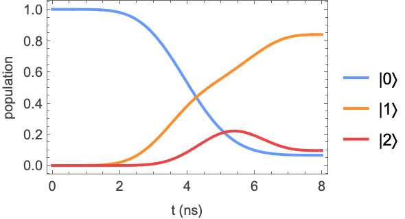
An 8 ns pulse without DRAG or detuning, starting from |0⟩:
In[8]:=
psi=
QuantumEvolve
[model[anharmonicity,0,0,8],FockState[0,5],{t,0,8}]
Out[8]=
QuantumState
Pure state
Qudits: 1
Type: Vector
Dimension: 5

The populations of the three lowest levels during the pulse:
In[9]:=
Plot[Evaluate[psi[t]["ProbabilitiesList"]〚;;3〛],{t,0,8},​​PlotStyle{StandardBlue,StandardOrange,StandardRed},​​PlotLegends{"|0〉","|1〉","|2〉"},​​FrameTrue,FrameLabel{"t (ns)","population"}]
Out[9]=
Population passes through |2⟩ on its way to |1⟩, and part of it stays there. At the end of the pulse 9.6% of the population is in |2⟩:
In[10]:=
psi[8]["ProbabilitiesList"]
Out[10]=
{0.0657671,0.838515,0.0956994,0.0000183186,1.90366×
-10
10
}
Pulses are compared through a function of the three controls. Numeric code here names them
drag
,
detuning
and
length
rather than
λ
,
δ
and
τ
:
Table
and
FindMinimum
localize their variables dynamically, so iterating over
τ
would also set it inside
model
. The final populations for a given DRAG coefficient, detuning and length:
In[11]:=
populations[drag_?NumericQ,detuning_?NumericQ,length_?NumericQ]:=​​
QuantumEvolve
[model[anharmonicity,drag,detuning,length],FockState[0,5],{t,0,length}][length]["ProbabilitiesList"]
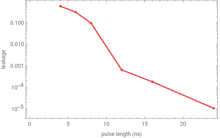
Leakage into |2⟩ for pulses from 4 to 24 ns:
In[12]:=
leakageTable=Table[{length,populations[0,0,length]〚3〛},{length,{4,6,8,12,16,24}}]
Out[12]=
{{4,0.583254},{6,0.30998},{8,0.0956994},{12,0.00064026},{16,0.000179682},{24,0.0000105546}}
On a logarithmic scale:
In[13]:=
ListLogPlot[leakageTable,JoinedTrue,MeshAll,PlotStyleStandardRed,​​FrameTrue,FrameLabel{"pulse length (ns)","leakage"}]
Out[13]=
Leakage falls by more than four orders of magnitude between 4 and 24 ns, but even at 24 ns a pulse without DRAG leaves 1.1 × 10⁻⁵ of the population in |2⟩.

DRAG

To first order in
1/α
, the DRAG quadrature removes the leakage at
λ
= 1. The transfer error counts the population that does not reach |1⟩, leakage included. Leakage and transfer error at 8 ns for
λ
= 0, 1/2 and 1:
In[14]:=
Table[With[{p=populations[drag,0,8]},{drag,p〚3〛,1-p〚2〛}],{drag,{0,1/2,1}}]
Out[14]=
{0,0.0956994,0.161485},
1
2
,0.0262962,0.0293745,{1,0.00116017,0.0810995}
λ
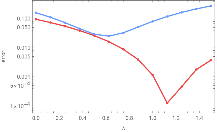
= 1 cuts the leakage by a factor of 80 but leaves 8% of the population short of |1⟩. A scan over
λ
shows the two errors reaching their minima at different values:
In[15]:=
ListLogPlot[​​Transpose@Table[With[{p=populations[drag,0,8]},{{drag,p〚3〛},{drag,1-p〚2〛}}],{drag,0,1.5,0.125}],​​JoinedTrue,MeshAll,PlotStyle{StandardRed,StandardBlue},​​PlotLegends{"leakage","transfer error"},FrameTrue,FrameLabel{"λ","error"}]
Out[15]=
leakage
transfer error
The best DRAG coefficient and detuning for a 12 ns pulse:

Decoherence and the Best Pulse Length

The pure dephasing time:
The transfer error with decay and dephasing, from the Lindblad master equation:
At the 12 ns optimum, decoherence adds 6 × 10⁻⁵:
With DRAG:
Without DRAG:
The error against pulse length, with and without DRAG:
Without DRAG:
DRAG roughly halves both the pulse length and its error, from 32 ns to 17.7 ns and from 2.0 × 10⁻⁴ to 9.8 × 10⁻⁵. The minimum without DRAG is flat. Started from 35 ns instead, the search stops at another length with almost the same error:
Its location is soft and its value is not.

Five Levels Are Enough

From three to six levels:
Three levels underestimate the leakage by almost half. Five and six agree to within 0.02%.

© 2026 Wolfram. All rights reserved.

  • Legal & Privacy Policy
  • Contact Us
  • WolframAlpha.com
  • WolframCloud.com