The Wolfram quantum framework handles many different quantum objects, including states, operators, channels, measurements, circuits, and more. It offers specialized functions for various computations like quantum evolution, entanglement monotones, partial tracing, Wigner or Weyl transformations, stabilizer formalism, and additional capabilities. Each functionality incorporates common named operations, such as Schwinger basis, GHZ state, Fourier operator, Grover circuit, and others. Perform computations seamlessly with the Wolfram quantum framework using the standard Wolfram kernel, such as the usual evaluation of codes in Mathematica. Alternatively, leverage the framework to send jobs to quantum processing units via service connections.
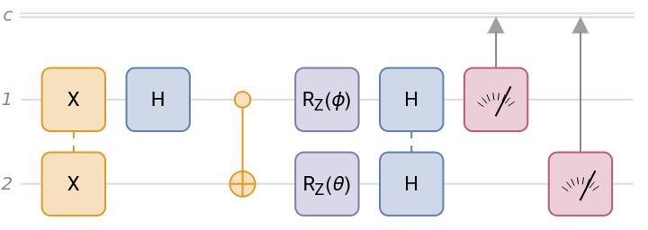
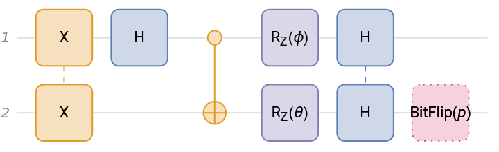
Create a quantum circuit composed of Pauli-X on qubits 1 and 2, Hadamard on qubit 1, CNOT with qubit 1 as the controlled and qubit 2 as the target, rotation around the z-axis by a symbolic angle ϕ on qubit 1, rotation around the z-axis by a symbolic angle θ on qubit 2, Hadamard on qubits 1 and 2, and finally, measurement in the computational basis on qubits 1 and 2.
Generate the multivariate distribution of measurement results based on the assumption that the angles are real:
Calculate the quantum correlation P00-P10-P01+P11
Calculate the state before measurements and show it in the Dirac notation:
Calculate the entanglement monotone of that state:
Add a bit-flip channel with a probability p only on the qubit-2:
Calculate the corresponding density matrix of the final quantum state of this circuit:
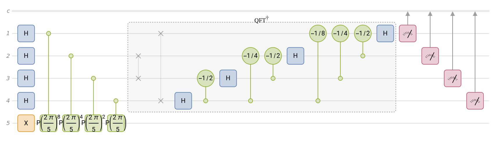
Create the quantum phase estimation circuit for a phase operator with a given angle and a given number of qubits:
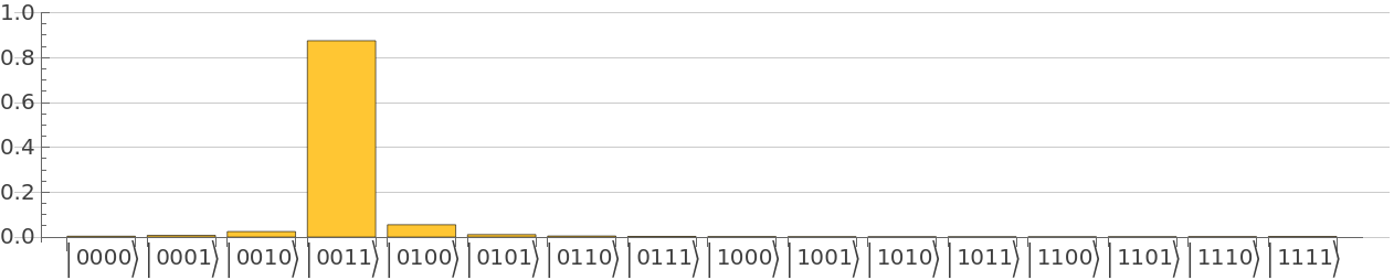
Calculate the outcome of circuit:
Calculate the corresponding probabilities:
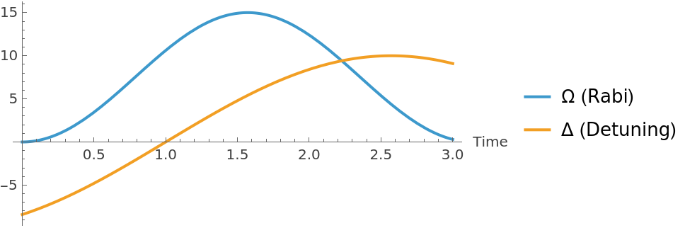
Set time and other variables of a Hamiltonian (Rabi drive and detuning):
Create a Hamiltonian operator as 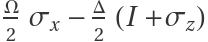
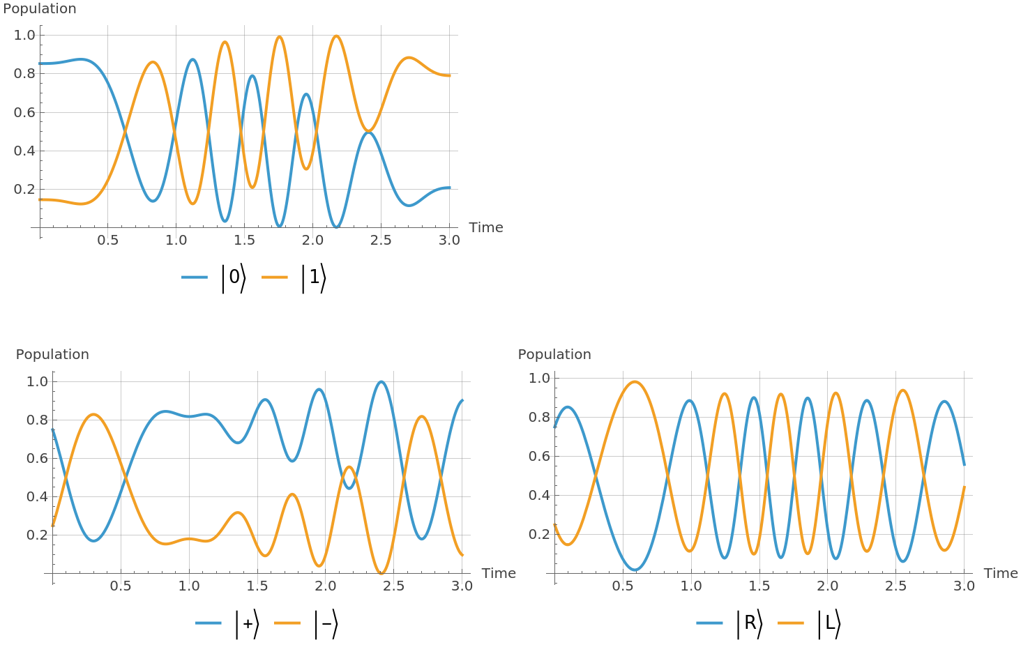
Evolve an initial quantum state using the Hamiltonian:
Plot the measurement probabilities in the different basis:
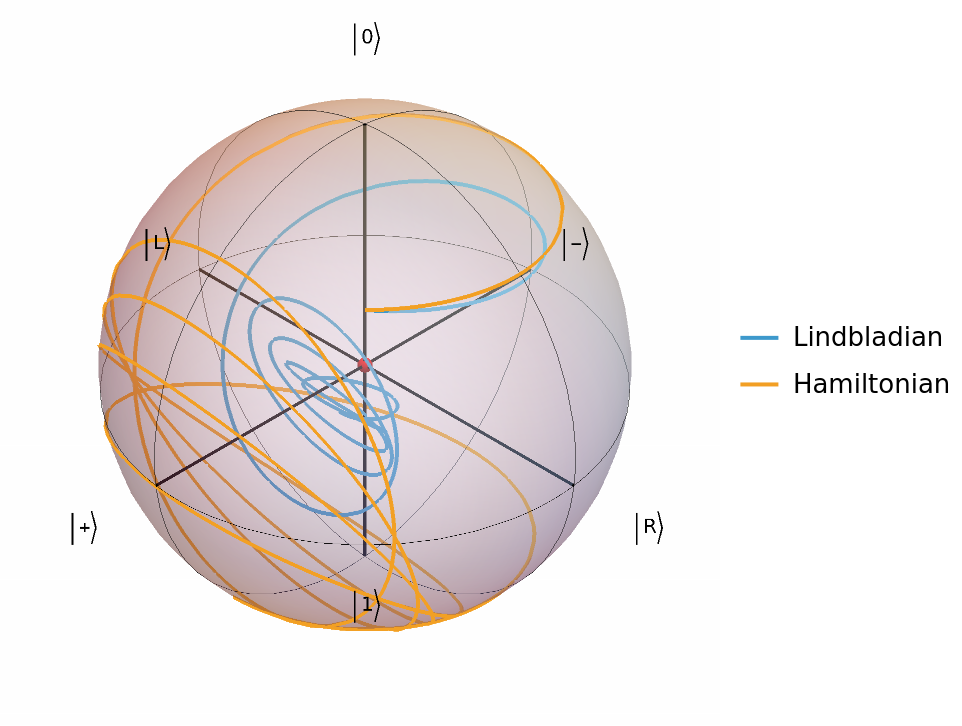
Plot the Bloch vector evolution:
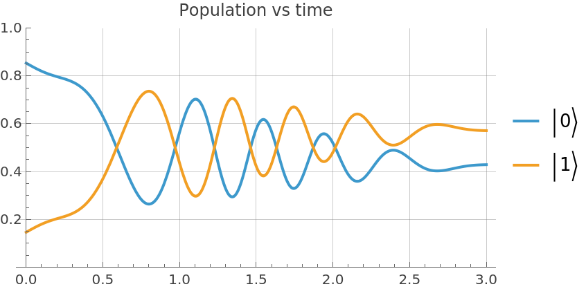
Define Lindblad operators (inducing jump from 1 to 0, and vice versa) with given rates:
Evolve the same initial state using the Lindblad equation:
Plot the measurement probabilities in the computational basis:
Plot the Bloch vector evolution vs the Hamiltonian one:

![\[CapitalOmega] = 15. Sin[t]^2;
\[CapitalDelta] = 10. Sin[t - 1];
Plot[{\[CapitalOmega], \[CapitalDelta]}, {t, 0, 3}, PlotLegends -> {"\[CapitalOmega] (Rabi)", "\[CapitalDelta] (Detuning)"},
AspectRatio -> 1/2, AxesLabel -> {"Time"}]](https://www.wolframcloud.com/obj/resourcesystem/images/b7a/b7acdc31-f5bd-43d2-a50f-580e75215231/68e758bf6a3aa678.png)
![Row[{Plot[Evaluate@Normal@\[Psi]["ProbabilitiesList"], {t, 0, 3.}, Sequence[PlotLegends -> Placed[{
Ket[{"0"}],
Ket[{"1"}]}, Bottom], AspectRatio -> 1/2, ImageSize -> Medium, GridLines -> Automatic, AxesLabel -> {"Time", "Population"}]], " ",
Plot[Evaluate@
Normal@InterpretationBox[FrameBox[TagBox[TooltipBox[PaneBox[GridBox[List[List[GraphicsBox[List[Thickness[0.0025`], List[FaceForm[List[RGBColor[0.9607843137254902`, 0.5058823529411764`, 0.19607843137254902`], Opacity[1.`]]], FilledCurveBox[List[List[List[0, 2, 0], List[0, 1, 0], List[0, 1, 0], List[0, 1, 0], List[0, 1, 0]], List[List[0, 2, 0], List[0, 1, 0], List[0, 1, 0], List[0, 1, 0], List[0, 1, 0]], List[List[0, 2, 0], List[0, 1, 0], List[0, 1, 0], List[0, 1, 0], List[0, 1, 0], List[0, 1, 0]], List[List[0, 2, 0], List[1, 3, 3], List[0, 1, 0], List[1, 3, 3], List[0, 1, 0], List[1, 3, 3], List[0, 1, 0], List[1, 3, 3], List[1, 3, 3], List[0, 1, 0], List[1, 3, 3], List[0, 1, 0], List[1, 3, 3]]], List[List[List[205.`, 22.863691329956055`], List[205.`, 212.31669425964355`], List[246.01799774169922`, 235.99870109558105`], List[369.0710144042969`, 307.0436840057373`], List[369.0710144042969`, 117.59068870544434`], List[205.`, 22.863691329956055`]], List[List[30.928985595703125`, 307.0436840057373`], List[153.98200225830078`, 235.99870109558105`], List[195.`, 212.31669425964355`], List[195.`, 22.863691329956055`], List[30.928985595703125`, 117.59068870544434`], List[30.928985595703125`, 307.0436840057373`]], List[List[200.`, 410.42970085144043`], List[364.0710144042969`, 315.7036876678467`], List[241.01799774169922`, 244.65868949890137`], List[200.`, 220.97669792175293`], List[158.98200225830078`, 244.65868949890137`], List[35.928985595703125`, 315.7036876678467`], List[200.`, 410.42970085144043`]], List[List[376.5710144042969`, 320.03370475769043`], List[202.5`, 420.53370475769043`], List[200.95300006866455`, 421.42667961120605`], List[199.04699993133545`, 421.42667961120605`], List[197.5`, 420.53370475769043`], List[23.428985595703125`, 320.03370475769043`], List[21.882003784179688`, 319.1406993865967`], List[20.928985595703125`, 317.4896984100342`], List[20.928985595703125`, 315.7036876678467`], List[20.928985595703125`, 114.70369529724121`], List[20.928985595703125`, 112.91769218444824`], List[21.882003784179688`, 111.26669120788574`], List[23.428985595703125`, 110.37369346618652`], List[197.5`, 9.87369155883789`], List[198.27300024032593`, 9.426692008972168`], List[199.13700008392334`, 9.203690528869629`], List[200.`, 9.203690528869629`], List[200.86299991607666`, 9.203690528869629`], List[201.72699999809265`, 9.426692008972168`], List[202.5`, 9.87369155883789`], List[376.5710144042969`, 110.37369346618652`], List[378.1179962158203`, 111.26669120788574`], List[379.0710144042969`, 112.91769218444824`], List[379.0710144042969`, 114.70369529724121`], List[379.0710144042969`, 315.7036876678467`], List[379.0710144042969`, 317.4896984100342`], List[378.1179962158203`, 319.1406993865967`], List[376.5710144042969`, 320.03370475769043`]]]]], List[FaceForm[List[RGBColor[0.5529411764705883`, 0.6745098039215687`, 0.8117647058823529`], Opacity[1.`]]], FilledCurveBox[List[List[List[0, 2, 0], List[0, 1, 0], List[0, 1, 0], List[0, 1, 0]]], List[List[List[44.92900085449219`, 282.59088134765625`], List[181.00001525878906`, 204.0298843383789`], List[181.00001525878906`, 46.90887451171875`], List[44.92900085449219`, 125.46986389160156`], List[44.92900085449219`, 282.59088134765625`]]]]], List[FaceForm[List[RGBColor[0.6627450980392157`, 0.803921568627451`, 0.5686274509803921`], Opacity[1.`]]], FilledCurveBox[List[List[List[0, 2, 0], List[0, 1, 0], List[0, 1, 0], List[0, 1, 0]]], List[List[List[355.0710144042969`, 282.59088134765625`], List[355.0710144042969`, 125.46986389160156`], List[219.`, 46.90887451171875`], List[219.`, 204.0298843383789`], List[355.0710144042969`, 282.59088134765625`]]]]], List[FaceForm[List[RGBColor[0.6901960784313725`, 0.5882352941176471`, 0.8117647058823529`], Opacity[1.`]]], FilledCurveBox[List[List[List[0, 2, 0], List[0, 1, 0], List[0, 1, 0], List[0, 1, 0]]], List[List[List[200.`, 394.0606994628906`], List[336.0710144042969`, 315.4997024536133`], List[200.`, 236.93968200683594`], List[63.928985595703125`, 315.4997024536133`], List[200.`, 394.0606994628906`]]]]]], List[Rule[BaselinePosition, Scaled[0.15`]], Rule[ImageSize, 10], Rule[ImageSize, 15]]], StyleBox[RowBox[List["QuantumState", " "]], Rule[ShowAutoStyles, False], Rule[ShowStringCharacters, False], Rule[FontSize, Times[0.9`, Inherited]], Rule[FontColor, GrayLevel[0.1`]]]]], Rule[GridBoxSpacings, List[Rule["Columns", List[List[0.25`]]]]]], Rule[Alignment, List[Left, Baseline]], Rule[BaselinePosition, Baseline], Rule[FrameMargins, List[List[3, 0], List[0, 0]]], Rule[BaseStyle, List[Rule[LineSpacing, List[0, 0]], Rule[LineBreakWithin, False]]]], RowBox[List["PacletSymbol", "[", RowBox[List["\"Wolfram/QuantumFramework\"", ",", "\"Wolfram`QuantumFramework`QuantumState\""]], "]"]], Rule[TooltipStyle, List[Rule[ShowAutoStyles, True], Rule[ShowStringCharacters, True]]]], Function[Annotation[Slot[1], Style[Defer[PacletSymbol["Wolfram/QuantumFramework", "Wolfram`QuantumFramework`QuantumState"]], Rule[ShowStringCharacters, True]], "Tooltip"]]], Rule[Background, RGBColor[0.968`, 0.976`, 0.984`]], Rule[BaselinePosition, Baseline], Rule[DefaultBaseStyle, List[]], Rule[FrameMargins, List[List[0, 0], List[1, 1]]], Rule[FrameStyle, RGBColor[0.831`, 0.847`, 0.85`]], Rule[RoundingRadius, 4]], PacletSymbol["Wolfram/QuantumFramework", "Wolfram`QuantumFramework`QuantumState"], Rule[Selectable, False], Rule[SelectWithContents, True], Rule[BoxID, "PacletSymbolBox"]][\[Psi], "X"][
"ProbabilitiesList"], {t, 0, 3.}, Sequence[
PlotLegends -> Placed[{
Ket[{"+"}],
Ket[{"-"}]}, Bottom], AspectRatio -> 1/2, ImageSize -> Medium, GridLines -> Automatic, AxesLabel -> {"Time", "Population"}]], Plot[Evaluate@
Normal@InterpretationBox[FrameBox[TagBox[TooltipBox[PaneBox[GridBox[List[List[GraphicsBox[List[Thickness[0.0025`], List[FaceForm[List[RGBColor[0.9607843137254902`, 0.5058823529411764`, 0.19607843137254902`], Opacity[1.`]]], FilledCurveBox[List[List[List[0, 2, 0], List[0, 1, 0], List[0, 1, 0], List[0, 1, 0], List[0, 1, 0]], List[List[0, 2, 0], List[0, 1, 0], List[0, 1, 0], List[0, 1, 0], List[0, 1, 0]], List[List[0, 2, 0], List[0, 1, 0], List[0, 1, 0], List[0, 1, 0], List[0, 1, 0], List[0, 1, 0]], List[List[0, 2, 0], List[1, 3, 3], List[0, 1, 0], List[1, 3, 3], List[0, 1, 0], List[1, 3, 3], List[0, 1, 0], List[1, 3, 3], List[1, 3, 3], List[0, 1, 0], List[1, 3, 3], List[0, 1, 0], List[1, 3, 3]]], List[List[List[205.`, 22.863691329956055`], List[205.`, 212.31669425964355`], List[246.01799774169922`, 235.99870109558105`], List[369.0710144042969`, 307.0436840057373`], List[369.0710144042969`, 117.59068870544434`], List[205.`, 22.863691329956055`]], List[List[30.928985595703125`, 307.0436840057373`], List[153.98200225830078`, 235.99870109558105`], List[195.`, 212.31669425964355`], List[195.`, 22.863691329956055`], List[30.928985595703125`, 117.59068870544434`], List[30.928985595703125`, 307.0436840057373`]], List[List[200.`, 410.42970085144043`], List[364.0710144042969`, 315.7036876678467`], List[241.01799774169922`, 244.65868949890137`], List[200.`, 220.97669792175293`], List[158.98200225830078`, 244.65868949890137`], List[35.928985595703125`, 315.7036876678467`], List[200.`, 410.42970085144043`]], List[List[376.5710144042969`, 320.03370475769043`], List[202.5`, 420.53370475769043`], List[200.95300006866455`, 421.42667961120605`], List[199.04699993133545`, 421.42667961120605`], List[197.5`, 420.53370475769043`], List[23.428985595703125`, 320.03370475769043`], List[21.882003784179688`, 319.1406993865967`], List[20.928985595703125`, 317.4896984100342`], List[20.928985595703125`, 315.7036876678467`], List[20.928985595703125`, 114.70369529724121`], List[20.928985595703125`, 112.91769218444824`], List[21.882003784179688`, 111.26669120788574`], List[23.428985595703125`, 110.37369346618652`], List[197.5`, 9.87369155883789`], List[198.27300024032593`, 9.426692008972168`], List[199.13700008392334`, 9.203690528869629`], List[200.`, 9.203690528869629`], List[200.86299991607666`, 9.203690528869629`], List[201.72699999809265`, 9.426692008972168`], List[202.5`, 9.87369155883789`], List[376.5710144042969`, 110.37369346618652`], List[378.1179962158203`, 111.26669120788574`], List[379.0710144042969`, 112.91769218444824`], List[379.0710144042969`, 114.70369529724121`], List[379.0710144042969`, 315.7036876678467`], List[379.0710144042969`, 317.4896984100342`], List[378.1179962158203`, 319.1406993865967`], List[376.5710144042969`, 320.03370475769043`]]]]], List[FaceForm[List[RGBColor[0.5529411764705883`, 0.6745098039215687`, 0.8117647058823529`], Opacity[1.`]]], FilledCurveBox[List[List[List[0, 2, 0], List[0, 1, 0], List[0, 1, 0], List[0, 1, 0]]], List[List[List[44.92900085449219`, 282.59088134765625`], List[181.00001525878906`, 204.0298843383789`], List[181.00001525878906`, 46.90887451171875`], List[44.92900085449219`, 125.46986389160156`], List[44.92900085449219`, 282.59088134765625`]]]]], List[FaceForm[List[RGBColor[0.6627450980392157`, 0.803921568627451`, 0.5686274509803921`], Opacity[1.`]]], FilledCurveBox[List[List[List[0, 2, 0], List[0, 1, 0], List[0, 1, 0], List[0, 1, 0]]], List[List[List[355.0710144042969`, 282.59088134765625`], List[355.0710144042969`, 125.46986389160156`], List[219.`, 46.90887451171875`], List[219.`, 204.0298843383789`], List[355.0710144042969`, 282.59088134765625`]]]]], List[FaceForm[List[RGBColor[0.6901960784313725`, 0.5882352941176471`, 0.8117647058823529`], Opacity[1.`]]], FilledCurveBox[List[List[List[0, 2, 0], List[0, 1, 0], List[0, 1, 0], List[0, 1, 0]]], List[List[List[200.`, 394.0606994628906`], List[336.0710144042969`, 315.4997024536133`], List[200.`, 236.93968200683594`], List[63.928985595703125`, 315.4997024536133`], List[200.`, 394.0606994628906`]]]]]], List[Rule[BaselinePosition, Scaled[0.15`]], Rule[ImageSize, 10], Rule[ImageSize, 15]]], StyleBox[RowBox[List["QuantumState", " "]], Rule[ShowAutoStyles, False], Rule[ShowStringCharacters, False], Rule[FontSize, Times[0.9`, Inherited]], Rule[FontColor, GrayLevel[0.1`]]]]], Rule[GridBoxSpacings, List[Rule["Columns", List[List[0.25`]]]]]], Rule[Alignment, List[Left, Baseline]], Rule[BaselinePosition, Baseline], Rule[FrameMargins, List[List[3, 0], List[0, 0]]], Rule[BaseStyle, List[Rule[LineSpacing, List[0, 0]], Rule[LineBreakWithin, False]]]], RowBox[List["PacletSymbol", "[", RowBox[List["\"Wolfram/QuantumFramework\"", ",", "\"Wolfram`QuantumFramework`QuantumState\""]], "]"]], Rule[TooltipStyle, List[Rule[ShowAutoStyles, True], Rule[ShowStringCharacters, True]]]], Function[Annotation[Slot[1], Style[Defer[PacletSymbol["Wolfram/QuantumFramework", "Wolfram`QuantumFramework`QuantumState"]], Rule[ShowStringCharacters, True]], "Tooltip"]]], Rule[Background, RGBColor[0.968`, 0.976`, 0.984`]], Rule[BaselinePosition, Baseline], Rule[DefaultBaseStyle, List[]], Rule[FrameMargins, List[List[0, 0], List[1, 1]]], Rule[FrameStyle, RGBColor[0.831`, 0.847`, 0.85`]], Rule[RoundingRadius, 4]], PacletSymbol["Wolfram/QuantumFramework", "Wolfram`QuantumFramework`QuantumState"], Rule[Selectable, False], Rule[SelectWithContents, True], Rule[BoxID, "PacletSymbolBox"]][\[Psi], "Y"][
"ProbabilitiesList"], {t, 0, 3.}, Sequence[
PlotLegends -> Placed[{
Ket[{"R"}],
Ket[{"L"}]}, Bottom], AspectRatio -> 1/2, ImageSize -> Medium, GridLines -> Automatic, AxesLabel -> {"Time", "Population"}]]}, Frame -> All]](https://www.wolframcloud.com/obj/resourcesystem/images/b7a/b7acdc31-f5bd-43d2-a50f-580e75215231/56d7039aa19eda3f.png)
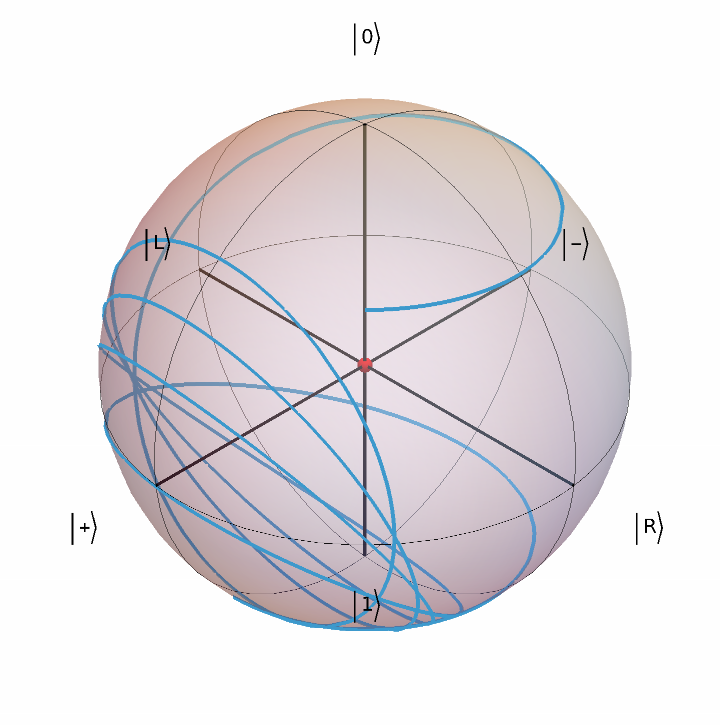
![Show[InterpretationBox[FrameBox[TagBox[TooltipBox[PaneBox[GridBox[List[List[GraphicsBox[List[Thickness[0.0025`], List[FaceForm[List[RGBColor[0.9607843137254902`, 0.5058823529411764`, 0.19607843137254902`], Opacity[1.`]]], FilledCurveBox[List[List[List[0, 2, 0], List[0, 1, 0], List[0, 1, 0], List[0, 1, 0], List[0, 1, 0]], List[List[0, 2, 0], List[0, 1, 0], List[0, 1, 0], List[0, 1, 0], List[0, 1, 0]], List[List[0, 2, 0], List[0, 1, 0], List[0, 1, 0], List[0, 1, 0], List[0, 1, 0], List[0, 1, 0]], List[List[0, 2, 0], List[1, 3, 3], List[0, 1, 0], List[1, 3, 3], List[0, 1, 0], List[1, 3, 3], List[0, 1, 0], List[1, 3, 3], List[1, 3, 3], List[0, 1, 0], List[1, 3, 3], List[0, 1, 0], List[1, 3, 3]]], List[List[List[205.`, 22.863691329956055`], List[205.`, 212.31669425964355`], List[246.01799774169922`, 235.99870109558105`], List[369.0710144042969`, 307.0436840057373`], List[369.0710144042969`, 117.59068870544434`], List[205.`, 22.863691329956055`]], List[List[30.928985595703125`, 307.0436840057373`], List[153.98200225830078`, 235.99870109558105`], List[195.`, 212.31669425964355`], List[195.`, 22.863691329956055`], List[30.928985595703125`, 117.59068870544434`], List[30.928985595703125`, 307.0436840057373`]], List[List[200.`, 410.42970085144043`], List[364.0710144042969`, 315.7036876678467`], List[241.01799774169922`, 244.65868949890137`], List[200.`, 220.97669792175293`], List[158.98200225830078`, 244.65868949890137`], List[35.928985595703125`, 315.7036876678467`], List[200.`, 410.42970085144043`]], List[List[376.5710144042969`, 320.03370475769043`], List[202.5`, 420.53370475769043`], List[200.95300006866455`, 421.42667961120605`], List[199.04699993133545`, 421.42667961120605`], List[197.5`, 420.53370475769043`], List[23.428985595703125`, 320.03370475769043`], List[21.882003784179688`, 319.1406993865967`], List[20.928985595703125`, 317.4896984100342`], List[20.928985595703125`, 315.7036876678467`], List[20.928985595703125`, 114.70369529724121`], List[20.928985595703125`, 112.91769218444824`], List[21.882003784179688`, 111.26669120788574`], List[23.428985595703125`, 110.37369346618652`], List[197.5`, 9.87369155883789`], List[198.27300024032593`, 9.426692008972168`], List[199.13700008392334`, 9.203690528869629`], List[200.`, 9.203690528869629`], List[200.86299991607666`, 9.203690528869629`], List[201.72699999809265`, 9.426692008972168`], List[202.5`, 9.87369155883789`], List[376.5710144042969`, 110.37369346618652`], List[378.1179962158203`, 111.26669120788574`], List[379.0710144042969`, 112.91769218444824`], List[379.0710144042969`, 114.70369529724121`], List[379.0710144042969`, 315.7036876678467`], List[379.0710144042969`, 317.4896984100342`], List[378.1179962158203`, 319.1406993865967`], List[376.5710144042969`, 320.03370475769043`]]]]], List[FaceForm[List[RGBColor[0.5529411764705883`, 0.6745098039215687`, 0.8117647058823529`], Opacity[1.`]]], FilledCurveBox[List[List[List[0, 2, 0], List[0, 1, 0], List[0, 1, 0], List[0, 1, 0]]], List[List[List[44.92900085449219`, 282.59088134765625`], List[181.00001525878906`, 204.0298843383789`], List[181.00001525878906`, 46.90887451171875`], List[44.92900085449219`, 125.46986389160156`], List[44.92900085449219`, 282.59088134765625`]]]]], List[FaceForm[List[RGBColor[0.6627450980392157`, 0.803921568627451`, 0.5686274509803921`], Opacity[1.`]]], FilledCurveBox[List[List[List[0, 2, 0], List[0, 1, 0], List[0, 1, 0], List[0, 1, 0]]], List[List[List[355.0710144042969`, 282.59088134765625`], List[355.0710144042969`, 125.46986389160156`], List[219.`, 46.90887451171875`], List[219.`, 204.0298843383789`], List[355.0710144042969`, 282.59088134765625`]]]]], List[FaceForm[List[RGBColor[0.6901960784313725`, 0.5882352941176471`, 0.8117647058823529`], Opacity[1.`]]], FilledCurveBox[List[List[List[0, 2, 0], List[0, 1, 0], List[0, 1, 0], List[0, 1, 0]]], List[List[List[200.`, 394.0606994628906`], List[336.0710144042969`, 315.4997024536133`], List[200.`, 236.93968200683594`], List[63.928985595703125`, 315.4997024536133`], List[200.`, 394.0606994628906`]]]]]], List[Rule[BaselinePosition, Scaled[0.15`]], Rule[ImageSize, 10], Rule[ImageSize, 15]]], StyleBox[RowBox[List["QuantumState", " "]], Rule[ShowAutoStyles, False], Rule[ShowStringCharacters, False], Rule[FontSize, Times[0.9`, Inherited]], Rule[FontColor, GrayLevel[0.1`]]]]], Rule[GridBoxSpacings, List[Rule["Columns", List[List[0.25`]]]]]], Rule[Alignment, List[Left, Baseline]], Rule[BaselinePosition, Baseline], Rule[FrameMargins, List[List[3, 0], List[0, 0]]], Rule[BaseStyle, List[Rule[LineSpacing, List[0, 0]], Rule[LineBreakWithin, False]]]], RowBox[List["PacletSymbol", "[", RowBox[List["\"Wolfram/QuantumFramework\"", ",", "\"Wolfram`QuantumFramework`QuantumState\""]], "]"]], Rule[TooltipStyle, List[Rule[ShowAutoStyles, True], Rule[ShowStringCharacters, True]]]], Function[Annotation[Slot[1], Style[Defer[PacletSymbol["Wolfram/QuantumFramework", "Wolfram`QuantumFramework`QuantumState"]], Rule[ShowStringCharacters, True]], "Tooltip"]]], Rule[Background, RGBColor[0.968`, 0.976`, 0.984`]], Rule[BaselinePosition, Baseline], Rule[DefaultBaseStyle, List[]], Rule[FrameMargins, List[List[0, 0], List[1, 1]]], Rule[FrameStyle, RGBColor[0.831`, 0.847`, 0.85`]], Rule[RoundingRadius, 4]], PacletSymbol["Wolfram/QuantumFramework", "Wolfram`QuantumFramework`QuantumState"], Rule[Selectable, False], Rule[SelectWithContents, True], Rule[BoxID, "PacletSymbolBox"]]["UniformMixture"][
"BlochPlot"], ParametricPlot3D[{\[Rho]["BlochVector"], \[Psi]["BlochVector"]}, {t, 0, 3}, PlotLegends -> {"Lindbladian", "Hamiltonian"}]]](https://www.wolframcloud.com/obj/resourcesystem/images/b7a/b7acdc31-f5bd-43d2-a50f-580e75215231/4b4f11122d8433c4.png)