Wolfram Language Paclet Repository

Community-contributed installable additions to the Wolfram Language

Primary Navigation

    • Cloud & Deployment
    • Core Language & Structure
    • Data Manipulation & Analysis
    • Engineering Data & Computation
    • External Interfaces & Connections
    • Financial Data & Computation
    • Geographic Data & Computation
    • Geometry
    • Graphs & Networks
    • Higher Mathematical Computation
    • Images
    • Knowledge Representation & Natural Language
    • Machine Learning
    • Notebook Documents & Presentation
    • Scientific and Medical Data & Computation
    • Social, Cultural & Linguistic Data
    • Strings & Text
    • Symbolic & Numeric Computation
    • System Operation & Setup
    • Time-Related Computation
    • User Interface Construction
    • Visualization & Graphics
    • Random Paclet
    • Alphabetical List
  • Using Paclets
    • Get Started
    • Download Definition Notebook
  • Learn More about Wolfram Language

QuantumFramework

Tutorials

  • Getting Started

Guides

  • Wolfram Quantum Computation Framework

Tech Notes

  • Bell's Theorem
  • Circuit Diagram
  • Exploring Fundamentals of Quantum Theory
  • QPU Service Connection
  • Quantum object abstraction
  • Quantum Optimization
  • Second Quantization Functions
  • Tensor Network
  • Quantum Computation

Symbols

  • EinsteinSummation
  • QuantumBasis
  • QuantumChannel
  • QuantumCircuitMultiwayGraph [EXPERIMENTAL]
  • QuantumCircuitOperator
  • QuantumDistance
  • QuantumEntangledQ
  • QuantumEntanglementMonotone
  • QuantumEvolve
  • QuantumMeasurement
  • QuantumMeasurementOperator
  • QuantumMeasurementSimulation
  • QuantumMPS [EXPERIMENTAL]
  • QuantumOperator
  • QuantumPartialTrace
  • QuantumPhaseSpaceTransform
  • QuantumShortcut [EXPERIMENTAL]
  • QuantumStateEstimate [EXPERIMENTAL]
  • QuantumState
  • QuantumTensorProduct
  • QuantumWignerMICTransform [EXPERIMENTAL]
  • QuantumWignerTransform [EXPERIMENTAL]
  • QuditBasis
  • QuditName
Tensor Network
QuantumCircuitOperator
[…]["TensorNetwork"]
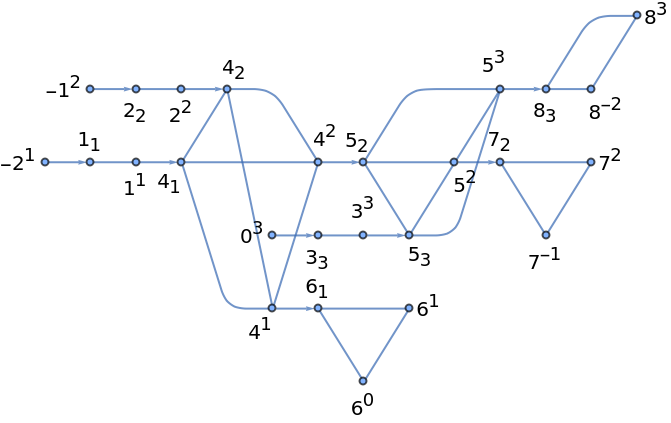
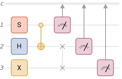
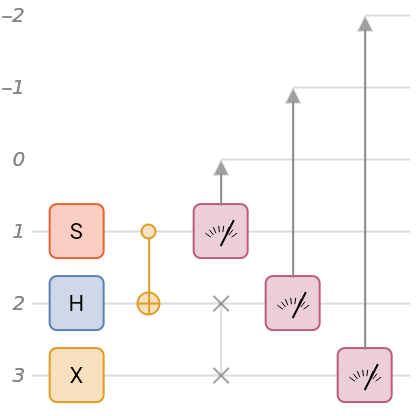
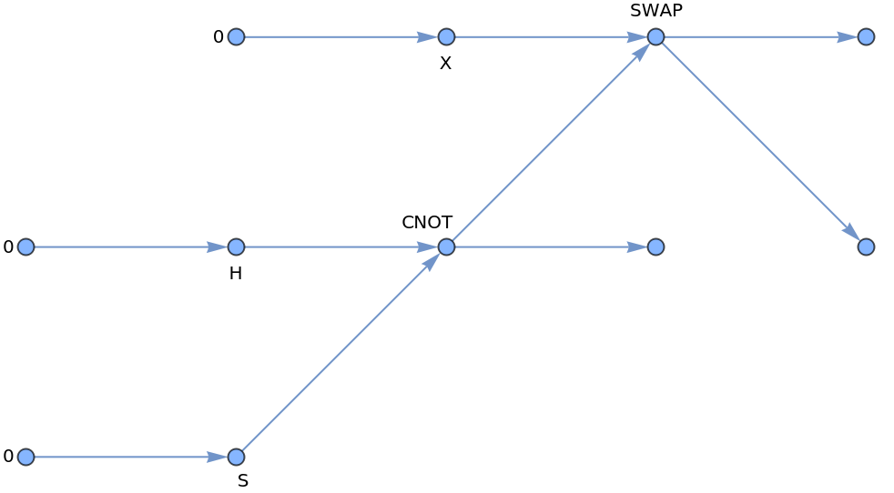
returns the tensor network of a circuit
TensorNetworkIndexGraph
[…]
transforms a tensor network into a new graph with indices as vertices
TensorNetworkFreeIndices
[…]
returns free indices in a tensor network index graph
ContractTensorNetwork
[…]
contracts indices in a tensor network
Create a quantum circuit:
In[84]:=
circuit=
QuantumCircuitOperator
[{"S","H"2,"X"3,"CNOT","SWAP"{2,3},{1},{2},{3}}];​​circuit["Diagram"]
Out[85]=
In the Wolfram Quantum Framework, measurement outcomes are recorded in an ancillary quantum register (serving as a detector), so the complete circuit diagram includes both the system and this detector subsystem.
In[86]:=
circuit["Diagram","ShowExtraQudits"True]
Out[86]=
The first measurement result is stored in wire index 0, with subsequent results assigned to decreasing (negative) wire indices.
Returns the tensor network representation corresponding to the given quantum circuit:
In[87]:=
net=circuit["TensorNetwork",GraphLayout{"LayeredDigraphEmbedding","Orientation"Left}]
Out[87]=
The tensor network is a graph annotated with tensors and contraction indices.
In[88]:=
GraphQ[net]&&TensorNetworkQ[net]
Out[88]=
True
For a graph to be a tensor network, two main conditions must be met, which is what
TensorNetworkQ
does. First, every vertex in the graph must have properly formatted indices consisting only of Subscript or Superscript expressions, and each vertex cannot contain any duplicate indices - all indices at any single vertex must be unique from each other.
Second, the tensor rank compatibility condition must be satisfied. This can happen in two ways: either each vertex's tensor rank must exactly match the number of indices assigned to that vertex, and when counting all index occurrences throughout the entire graph, every distinct index must appear exactly twice across all vertices (ensuring proper pairing for tensor contraction), or alternatively, all tensors in the network must have rank zero representing scalar tensors with no indices.
Lists all annotation keys available for the tensor network:
In[89]:=
AnnotationKeys[{net,0}]
Out[89]=
{Index,Tensor,VertexCoordinates,VertexLabels,VertexShape,VertexShapeFunction,VertexSize,VertexStyle}
Let’s look at tensor, vertex labels, and corresponding indexes in the tensor network:
Out[97]//TableForm=
Vertex index -> Vertex label
Tensor
Leg indices
-20
SparseArray
Specified elements: 1
Dimensions: {2}

{
1
-2
}
-10
SparseArray
Specified elements: 1
Dimensions: {2}

{
2
-1
}
00
SparseArray
Specified elements: 1
Dimensions: {2}

{
3
0
}
1S
SparseArray
Specified elements: 2
Dimensions: {2,2}

{
1
1
,
1
1
}
2H
SparseArray
Specified elements: 4
Dimensions: {2,2}

{
2
2
,
2
2
}
3X
SparseArray
Specified elements: 2
Dimensions: {2,2}


3
3
,
3
3

4CNOT
SparseArray
Specified elements: 4
Dimensions: {2,2,2,2}

{
1
4
,
2
4
,
4
1
,
4
2
}
5SWAP
SparseArray
Specified elements: 4
Dimensions: {2,2,2,2}


2
5
,
3
5
,
5
2
,
5
3

6None
SparseArray
Specified elements: 2
Dimensions: {2,2,2}

{
0
6
,
1
6
,
6
1
}
7None
SparseArray
Specified elements: 2
Dimensions: {2,2,2}

{
-1
7
,
2
7
,
7
2
}
8None
SparseArray
Specified elements: 2
Dimensions: {2,2,2}


-2
8
,
3
8
,
8
3

Tensors in the tensor network are mixed type, meaning they consist of so-called “contravariant” (upper) indices and “covariant” (lower) indices. For example, the 2nd measurement (7th vertex), acts on qubit-2 (denoted by contravariant and covariant indices 2) and its result is saved on wire, denoted by the index “-1”.
Vertices correspond to circuit’s operators/gate indices, in addition to “Initial” tensor with index 0 (for the initial state):
In[98]:=
VertexList[net]
Out[98]=
{-2,-1,0,1,2,3,4,5,6,7,8}
In[99]:=
Length@circuit["Flatten"]["Operators"]
Out[99]=
8
In[100]:=
%Max[%%]
Out[100]=
True
Note that each edge represents (i.e., is tagged by) a contraction:
In[101]:=
EdgeList[net]
Out[101]=
-2

1
-2
,
1
1


1,-1

2
-1
,
2
2


2,0

3
0
,
3
3


3,1

1
1
,
4
1


4,2

2
2
,
4
2


4,4

2
4
,
5
2


5,3

3
3
,
5
3


5,4

1
4
,
6
1


6,5

2
5
,
7
2


7,5

3
5
,
8
3


8
Corresponding contraction:
In[102]:=
EdgeTags[net]
Out[102]=
{
1
-2
,
1
1
},{
2
-1
,
2
2
},
3
0
,
3
3
,{
1
1
,
4
1
},{
2
2
,
4
2
},{
2
4
,
5
2
},
3
3
,
5
3
,{
1
4
,
6
1
},{
2
5
,
7
2
},
3
5
,
8
3

Perform the contraction:
In[103]:=
finalTensor=ContractTensorNetwork[net]
Out[103]=
SparseArray
Specified elements: 2
Dimensions: {2,2,2,2,2,2}

Confirm that the result is the same as default circuit application:
In[104]:=
circuit[]["Tensor"]finalTensor
Out[104]=
True
Another tensor network representation uses indices as graph vertices with tensors as cliques:
In[105]:=
indexNet=TensorNetworkIndexGraph[net,GraphLayout{"LayeredDigraphEmbedding","Orientation"Left}]
Out[105]=
In the above graph, the directed edges imply tensor contraction; also tensors are cliques in above graph:
In[106]:=
HighlightGraph[indexNet,Subgraph[indexNet,#]&/@FindClique[indexNet,Infinity,All]]
Free indices are the ones that left after contraction:
Highlight free indices:
Free indices can be extracted as vertices with zero in- and out- degree:

Contraction and Einstein Summation

Many useful information of a tensor network can be extracted using TensorNetworkData:
Also, one can get the useful data using graph functionalities, too:
Show ContractTensorNetwork is the same as EinsteinSummation:
One can compare the performance, on how the relevant computation is done
Perform the contraction in the order of network’s EdgeList:
Optimize the order for contraction, using EinsteinSummation and symbolic tensors package:

Initial state different from ground state

Note that the initial tensor in the tensor network we studied here was a registered state. Additionally, one can start from any initial state.
Generate a random state:
Initialize the tensor network from above state:
See supplement info, for package-scoped symbols.
Show the tensor contraction is the same as transformation of state by the circuit:
Supplement info

FromTensorNetwork

Any directed graph can be turned into a tensor network, even if the graph is not annotated.
Get the tensor network data:
One can assign symbolic tensor into vertices too:

Package-scoped symbols

© 2025 Wolfram. All rights reserved.

  • Legal & Privacy Policy
  • Contact Us
  • WolframAlpha.com
  • WolframCloud.com