Wolfram/QuantumFramework | Paclet Repository

Quantum Optimization

Variational Quantum Algorithms	Quantum Natural Gradient Descent
Variational Circuits	Quantum Linear Solver
Variational Quantum Eigensolver (VQE)	Classiq Integration
Quantum Approximate Optimization Algorithm (QAOA)

This technical note presents documentation for the functionalities utilized in the implementation of quantum optimization algorithms. The document systematically outlines the core features, methodologies, and application contexts of the framework, offering insights into its integration within the quantum computational paradigm.

By providing a comprehensive overview and usage guidelines for these functions, we aim to introduce new and experienced users into quantum optimization techniques and quantum computing research.

In[1]:=

<<Wolfram`QuantumFramework`<<Wolfram`QuantumFramework`QuantumOptimization`

Variational Quantum Algorithms

Introduction

Quantum computing has long been envisioned as a transformative technology, with the potential to tackle problems that are intractable for classical computers. Quantum algorithms promise exponential speedups in areas such as number factorization, quantum system simulation, and solving linear systems of equations.

The introduction of cloud-based quantum computers in 2016 provided public access to real quantum hardware. However, due to noise and the limited number of qubits, running large-scale quantum algorithms remained impractical. This led to growing interest in what could be achieved with these early devices, commonly referred to as Noisy Intermediate-Scale Quantum (NISQ) computers. Today’s state-of-the-art NISQ devices contain up to 1000 qubits, with only two quantum processors having over 1,000 qubits, making it possible to surpass classical supercomputers in specific, carefully designed computational tasks—a milestone known as quantum supremacy.

Variational Quantum Algorithms (VQAs) have emerged as the leading approach for using the power of NISQ devices. Given the constraints of current quantum hardware, VQAs employ a hybrid quantum-classical optimization framework. They utilize parameterized quantum circuits executed on a quantum computer, while classical optimizers adjust the parameters to minimize a given cost function. This strategy mirrors machine-learning techniques, such as neural networks, which rely on optimization-based learning methods.

Applications

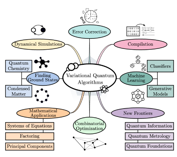
VQAs have been explored for a wide range of applications, spanning nearly all areas initially envisioned for quantum computing. As illustrated in the following image, VQAs are applied across various domains, including error correction, machine learning, combinatorial optimization, ground-state estimation, and mathematical problem-solving.

Cerezo, M., Arrasmith, A., Babbush, R. et al. Variational quantum algorithms. Nat Rev Phys 3, 625–644 (2021)

While they hold promise for achieving near-term quantum advantage, significant challenges remain, including issues related to trainability, accuracy, and efficiency. Addressing these challenges is crucial for the continued advancement of VQAs and their practical implementation in solving real-world problems.

In simple terms, Variational Quantum Algorithms (VQAs) are one of the most popular approaches for running quantum algorithms on today’s early-stage quantum computers. You can think of VQAs like “putting the carriage before the horses”, we know what problem we want to solve, but we don’t yet know the exact quantum circuit to do it. Instead of designing the circuit manually, VQAs use classical optimization techniques to “learn” the best circuit for the task.

Pipeline

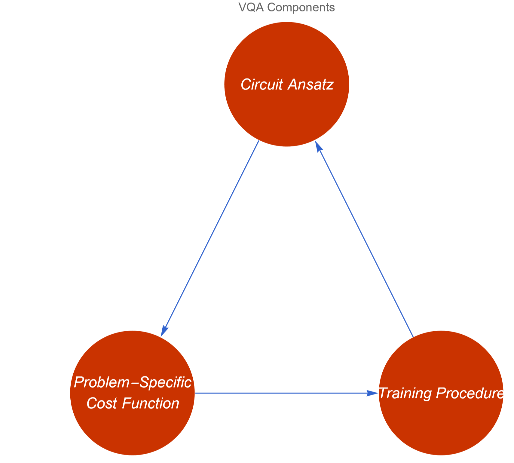
The core components of this algorithms include a parameterized quantum circuit, known as the ansatz, which is used to represent possible solutions. This ansatz is evaluated through a cost function that encodes the problem we are trying to solve. Finally, a training procedure, primarily driven by a classical optimizer, adjusts the parameters of the ansatz to improve the solution iteratively.

Out[15]=

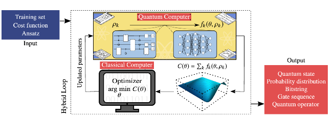
This process is best illustrated in the Hybrid Loop shown in the next image. The quantum computer runs the ansatz, the results are evaluated through the cost function, and the classical optimizer processes this information to update the parameters for the next iteration.

Cerezo, M., Arrasmith, A., Babbush, R. et al. Variational quantum algorithms. Nat Rev Phys 3, 625–644 (2021)

Now, rather than just describing it, let’s dive into parametrized circuits!

Variational Circuits

The area of Quantum Optimization depends heavily in variational algorithms. This algorithms work by exploring and comparing variational states

|ϕ(θ)〉

that depends on a set of

{θ}

parameters.

You can build this variational states using a fixed initial state as

|0〉

and a parametrized or variational quantum circuit

V(θ)

|ϕ(θ)〉=V(θ)|0〉

We aim to train these variational quantum circuits using an optimizer in conjunction with a cost function that reflects the objective of our optimization. Many of the algorithms presented here are Hybrid Algorithms, meaning they combine a quantum circuit with a classical optimizer.

Wolfram Quantum Framework supports "free parameters" in their quantum circuits. In order to implement a variational quantum circuit, you only need to specify this tunable parameters by using the "Parameters" option:

In[3]:=

vqc=

QuantumCircuitOperator

[{"00","RX"[θ1]{1},"RY"[θ2]{2}},"Parameters"{θ1,θ2}];

In[100]:=

vqc["Diagram"]

Out[100]=

The parameters defined for a Wolfram Quantum Framework Operator are heritable, so you do not need to redefine it in later steps. For example we can calculate the resultant

|ϕ(θ)〉

state from our defined variational circuit:

In[4]:=

vqs=vqc[]

Out[4]=

QuantumState

Pure state	Qudits: 2
Type: Vector	Dimension: 4



We can verify that the "Parameters" option values:

In[5]:=

vqs["Parameters"]

Out[5]=

{θ1,θ2}

This option simplifies the repeated execution of the circuit by using the symbolic computation capabilities provided by the Wolfram Quantum Framework:

In[6]:=

vqc["Formula"]

Out[6]=

Cos

θ1

Cos

θ2

|00〉+Cos

θ1

Sin

θ2

|01〉-Cos

θ2

Sin

θ1

|10〉-Sin

θ1

Sin

θ2

|11〉

Replace θ1 value as follows:

In[7]:=

vqc[θ10]["Formula"]

Out[7]=

Cos

θ2

|00〉+Sin

θ2

|01〉

As mentioned earlier, you can use the parameters at any stage of your algorithm, as they are carried through each step:

In[91]:=

vqs["Formula"]

Out[91]=

Cos

θ1

Cos

θ2

|00〉+Cos

θ1

Sin

θ2

|01〉-Cos

θ2

Sin

θ1

|10〉-Sin

θ1

Sin

θ2

|11〉

In[8]:=

vqs[θ20,θ10]["Formula"]

Out[8]=

|00〉

You can directly replace the values for each parameter following the same order you defined them:

In[95]:=

vqs[0,0]["Formula"]

Out[95]=

|00〉

In[99]:=

vqs[a,b]["Formula"]

In the following sections, we will explore variational algorithms, which will require an understanding of how to properly design (ansatz circuits) and train (classical optimizers) these variational circuits.

Initial State Preparation

If you have an educated guess or an existing optimal solution, using it as the reference state can help the variational algorithm converge faster.

The simplest reference state is the default state, where we initialize an n-qubit quantum circuit in the all-zero state:

For this default state, our unitary operator is simply the identity operator. Due to its simplicity, this default state is widely used as a reference state in many applications.

If we want to start with a more complex reference state that involves superposition and entanglement, we can prepare a state such as:

Which is also called a Bell State:

Ansatz Circuits

In physics and mathematics, the German word “Ansatz” refers to an educated guess for solving a problem. You may have done this before—trying out a potential solution based on intuition or prior knowledge. However, an ansatz is not just any guess; it must be well-informed.

In Variational Quantum Algorithms (VQAs), what we are guessing is the quantum circuit that will solve our problem. This is why we refer to this circuit simply as the ansatz

Generate a collection of parametrized states:

How Do We Choose an Ansatz?

◼

Problem-Inspired Ansatz

◼

If we have prior knowledge about the problem, we can use physical intuition or mathematical insights to design a circuit tailored to the task. This approach typically leads to more efficient circuits with fewer parameters, making optimization easier. These are usually referred to generally as Hardware-Efficient ansatz.

◼

Problem-Agnostic Ansatz

◼

If we lack detailed knowledge about the problem, we can use a more general universal ansatz that does not rely on problem-specific intuition. These ansatze are more expressive, meaning they can represent a wide range of solutions. However, they also tend to be larger, with more gates and parameters, making the optimization process significantly harder.

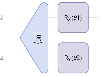
If we consider this simple ansatz, consisting of a pair of rotations and a CNOT gate, we can evaluate it and examine the states that can be generated:

As we observe, the possible states generated by this ansatz are limited to those determined by the sine and cosine functions. Therefore, even with an excellent optimizer, there will be certain values that this ansatz will never be able to reach:

How good is an ansatz?

◼

Expressibility

◼

This measures the range of functions that the quantum circuit can represent. Higher expressibility is generally linked to more entanglement and a greater number of parameters. The more expressive an ansatz is, the more problems it can potentially solve.

◼

Trainability

◼

This refers to how easy it is to find the right parameters for the circuit. Larger, highly expressive circuits are harder to optimize because the optimizer must explore a vast parameter space. The difficulty of training also depends on the cost function and the classical optimizer used.

There is a natural trade-off between expressibility and trainability. Highly expressive circuits are powerful but harder to train, while simpler circuits may be easier to optimize but might not capture the necessary complexity of the problem.

The goal is to find an ansatz in the “sweet spot”—one that is expressive enough to solve the problem but still trainable within a reasonable amount of time.

Now, let’s explore this concept further with an exercise!

◼

Exercise 1:

Express the collection of parametrized states generated by the following ansatz:

Step by step:

◼

Exercise 2:

Express the collection of parametrized states generated by the following ansatz:

Following the same steps:

We can verify that the second ansatz has more expressibility by the simple fact that:

The first ansatz is a specific case of the second ansatz:

Layered Circuit Architecture

What happens if we have no idea about the problem solution?

Layered gate architectures, where the ansatz is repeated multiple times, have been shown to offer a good balance between expressibility and relatively low circuit depth, making them effective for tackling a broad range of problems.

If the problem we are trying to solve doesn’t require a large number of parameters, a good option might be to use an ansatz called the Basic Entangler. This ansatz is often favored for its simplicity and efficiency in cases where the problem doesn’t demand an overly complex parameterized quantum circuit. This layers consist of one-parameter single-qubit rotations on each qubit, followed by a closed chain or ring of CNOT gates.

In order to generate multiple layers of parametrized gates or controlled gates you can use the following functionalities:

ParametrizedLayer & GenerateParameters

ParametrizedLayer

The ParametrizedLayer function reduces redundant code in layered quantum circuit architectures by applying parameterized gates and automatically generating the necessary parameters.

It is possible to specify both the qubits on which the parameterized gates will be applied and the index for each parameter:

Alternatively, you can specify only the parameter indices, and the gates will be generated sequentially for each qubit, starting from qubit 1:

GenerateParameters

The GenerateParameters function generates a list of symbols; you only need to specify the number of qubits and layers in the quantum circuit:

Example

Options

GenerateParameters and ParametrizedLayer functions use "θ" as default symbol:

Use "Symbol" option to change the default symbol:

EntanglementLayer

The EntanglementLayer function is designed to reduce redundant code in layered quantum circuit architectures by facilitating controlled operations between qubits.

The EntanglementLayer function returns a Sequence of multiple Rules, each representing a controlled gate applied to connected qubits according to the chosen entanglement strategy. Currently, the function supports only named controlled gates between two qubits.

Entanglement

The "Entanglement" option specifies the strategy used for entanglement. It supports the following values:

The variational quantum eigensolver (VQE) is a hybrid algorithm that combines classical and quantum computing to determine the ground state energy of a Hamiltonian. It utilizes quantum algorithms to calculate expected energy values and classical optimization techniques for minimizing that energy.

VQE plays a crucial role in quantum optimization, particularly in solving complex problems in quantum chemistry and materials science. By enabling efficient simulations of intricate systems, VQE can address optimization tasks that are challenging for classical methods alone.

Given a Hamiltonian operator H, this method consist of two main components:

The method involves iteratively adjusting θ to minimize the average energy or cost function .

Implementation

Define the ansatz circuit V(θ):

Implement the cost function ℒ as stated before:

Calculate the ground state eigenvalue of H by minimizing :

Visualizations

In order to visualize the optimization process, we need to get all the parameter values during the evolution, in this case we will use a simple gradient descent method:

It would be also useful to calculate all the cost function values during each step of the parameter evolution:

Cost curve

We can visualize the evolution of our optimization during time in an Cost Curve, also known as Loss Curve:

Parameter Space

We can visualize the evolution of our optimization in the parameter space in a Contour Plot:

Gradient Vector Plot

The stream plot of the gradient of our cost function can provide insight into the behavior of the evolution as observed in its parameter space:

Quantum Chemistry

The Variational Quantum Eigensolver (VQE) is a valuable tool in quantum chemistry for finding the minimal energy of a molecule. The task is essentially an optimization problem, where the goal is to minimize the total energy of the molecule with respect to the positions of the atomic nuclei.

In the case of VQE, we use parameterized quantum circuits to approximate the ground state energy of the system. This results in the determination of the minimal energy of the system, which corresponds to the lowest energy configuration of the molecule in its ground state.

This minimal energy result can be incredibly useful in determining the geometry of the molecule as well, as the lowest energy corresponds to the optimized configuration of the atomic nuclei. Therefore, although the main goal is to minimize the energy, this process can also provide insights into the stable arrangement of atoms in the molecule.

Implement the algorithm as we learned last class:

◼

First: Parametrized quantum circuits, state and ansatz preparation.

In this case we will use a typical hardware-efficient ansatz: Two layers of Rotations and a CNOT to ensure the entanglement.

We need a cost function, so let’s obtain the QuantumState from the QuantumCircuit and define the bra and ket.

Finally lets compute the energy of our system and define a function that will work as the cost function. In this step we should help the optimizer by Simplifying and replacing fixed values.

As I mentioned, the cost function we are working with is not trivial, but the advantage is that we can compute it symbolically, which significantly helps in the optimization process.

◼

Third: Optimization

To find the optimal parameters for our quantum circuit, we can use the NMinimize function in Mathematica.

This function allows us to minimize the cost function by adjusting the parameters, and after performing this minimization, we obtain the optimized parameters and the minimum value of the cost function, which in this case is approximately -0.824.

Now that we have the optimal value, it is insightful to inspect the behavior of the cost function around these points. Since we have four variables (the parameters in the ansatz), we need to fix two of the values in order to visualize the function.

We can do this by using a ContourPlot, which will allow us to observe the shape of the cost function in two dimensions.

ContourPlot is useful here because it highlights where the cost function attains higher and lower values. In this plot, the lighter sections correspond to higher values, and the blue sections represent the lowest values of the cost function.

If the optimization algorithm has started with a point near the blue section (where the minimum lies), we can expect it to converge towards this blue region, as this represents the optimal set of parameters. The algorithm searches for regions where the cost is minimized, and this plot helps visualize the “shape” of the function.

When the cost function is relatively simple and can be expressed symbolically, the ContourPlot can exhibit repetitive patterns. This repetition often results from the periodic nature of trigonometric functions (e.g., sin⁡and cos) that may appear in the cost function due to the rotation gates used in the ansatz.

Example from https://arxiv.org/pdf/1909.05074v1

Trihydrogen cation

First we will use some python code from PennyLane to obtain the Hamiltonian corresponding to the H3 cation.

We just need to indicate the molecules “H” and the coordinates:

〉

In[4]:=

import pennylane as qml
from pennylane import numpy as np

symbols = ["H", "H", "H"]
coordinates = np.array([0.028, 0.054, 0.0, 0.986, 1.610, 0.0, 1.855, 0.002, 0.0])

# Building the molecular hamiltonian for the trihydrogen cation
hamiltonian, qubits = qml.qchem.molecular_hamiltonian(symbols, coordinates, charge=1)

qml.matrix(hamiltonian)

In case Python is not available, you can import it from this location:

Finally we obtain a NumericArray which we will turn into a QuantumOperator:

If we have no prior knowledge of the structure of the circuit, a reasonable starting point could be a layered circuit consisting of rotations around the Y-axis and CNOT gates.

To encode the occupation numbers of the molecular spin-orbitals, we would need six qubits.

In this case, you can expect a very complex symbolic cost function. To handle this, we could choose to implement a numerical function instead.

We begin by using Module to define the quantum state with parameters replaced by real numbers. Next, we define the ket and bra, and then compute the scalar resulting from the expectation value of the Hamiltonian H.

After defining the cost function, we can apply a classical optimizer starting from an initial guess to find the minimum energy value.

If we are interested in obtaining the geometry of the system, we would need to introduce a parameterized Hamiltonian for optimization as well, to optimize both the energy and the geometry.

Quantum Approximate Optimization Algorithm (QAOA)

The Quantum Approximate Optimization Algorithm (QAOA) is a well-studied approach for solving combinatorial optimization problems.

The QAOA process involves the following steps:

◼

Defining the Oracles:

◼

Applying the Oracles alternately in layers, forming the unitary:

Quantum Combinational Optimization

The combinatorial optimization problem involves finding an optimal solution from a finite set of possibilities. This problem can be formulated as maximizing an objective function, which is expressed as a sum of Boolean functions.

For a problem with n bits and m clauses, the goal is to find a n-bit string z that maximizes the function:

Approximate optimization aims to find a near-optimal solution to this problem, which is often NP-hard. The approximate solution is an n-bit string z that closely maximizes the objective function 𝐶(t).

Max-Cut Problem

The Max–Cut problem is a well-known optimization problem in graph theory. The Maximum Cut problem involves partitioning the set of vertices V of a graph into two disjoint subsets, such that the number of edges connecting nodes in different subsets is maximized.

Formulating Max-Cut with Classical Binary Variables

Solve the classical Max-Cut problem:

This follows the solution given in the first image:

Formulating Max-Cut with Quantum Mechanics

To solve the Max-Cut problem on a quantum computer, we need to reformulate it in terms of quantum mechanics. Specifically, we convert the classical optimization problem into one of finding the eigenstate of a quantum Hamiltonian.

Our goal now shifts from finding a binary string to identifying the highest-energy eigenstate of a quantum Hamiltonian.

where:

We just need to express the summatory and for each term indicate which qubits are connected with a Z operator.

Represent each node as a qubit, then we have the bitstring:

Understanding QAOA Ansatz

To implement the Max-Cut problem on a quantum computer, we start by putting the nodes in superposition. This ensures that each node (qubit) has an equal probability of being in either partition.

Some initial intuition comes from our first example, which involves identifying a periodic pattern, such as 0101 or 1010, within a bitstring.

To achieve this, we need to establish connections between nodes or qubits that reflect the structure of the cost Hamiltonian. For this initial idea, we can evaluate the gate sequence CNOT + RZ + CNOT.

We can verify that it distinguish the possible correct solutions from the non-periodic bitstrings in order to solve the problem:

We can gain some initial insights and visualize the differences in the solution amplitudes in the following plot:

The concept becomes clearer when we observe that the probabilities of regular bitstrings are minimal when the probabilities of periodic bitstrings are maximal, and vice versa:

The set of gates outlined earlier is commonly referred to as an RZZ gate, which combines rotations and controlled operations:

Now that we understand this, we can apply it to every pair of qubits connected in the graph. In other words, we apply the RZZ gate to every edge in the graph. This ensures that the quantum state evolves according to the problem constraints.

The previous step does not explore all possible cuts because some amplitudes remain unchanged, so we need to mix things a little bit!

Visualize the symbolic function corresponding to each possible state:

Considering the initial state preparation, we recover a mini-QAOA:

The increased expressibility of the resulting state from this ansatz, as compared to previous circuits, comes from the final mixing performed by the mixing layer of gates:

From the following plot, we can observe how the probabilities for regular and periodic bitstrings oscillate, similar to the previous plots. The new parameter θ does not interfere with this behavior; instead, it expands the parameter space, providing additional expressibility to our ansatz:

Step–by–Step: 4-Edge Graph Example

Find the Max-Cut for the following graph:

Implement the Cost Hamiltonian:

Initial state preparation for superposition:

We can use Wolfram Mathematica's Graph functionalities to establish connections between qubits within the Cost-Circuit:

This layer of gates actually corresponds to the operator generated by the Cost Hamiltonian we defined earlier:

To ensure full exploration, we need a mixer Hamiltonian that allows transitions between different states:

Define the variational states to calculate the Cost function:

Let's try out the NMaximize optimizer:

We can enhance the precision of our solution by increasing the number of QAOA layers. This is easy to do since we can use QuantumCircuitOperator with the previous circuit but replacing the parameters:

We can utilize the Parameters option from the Wolfram Quantum Framework to re-name the gate parameters, allowing us to distinguish one layer from another.

Implement the cost function:

Optimimize:

Now, we obtain the exact result.

This solution represents the cut shown in the first image of this section:

Example: 5-Edge Graph

With a clear understanding of each step involved in solving the Max-Cut problem using QAOA, we are now ready to proceed with the direct implementation of the solution.

Find the Max-Cut for the following graph:

In this more challenging example, we will generate the Hamiltonian programmatically instead of writing it explicitly:

Implement directly the QAOA circuit using the Graph functionalities:

Implement the symbolic cost function using the Cost Hamiltonian and the resulting parametrized state from the previous circuit:

Use NMaximize for the optimization:

We obtain multiple possible solutions; however, with just a single QAOA layer, we observe four solutions with higher probability:

Solve it clasically:

The quantum algorithm does not achieve the maximum value compared to the classical solution, but we can analyze the four most probable solutions indicated by the ProbabilityPlot:

Example: 6-Edge Graph

Find the Max-Cut for the following graph:

In this more challenging example, we have a graph with six nodes, which results in a much larger cost Hamiltonian:

Implement directly the QAOA circuit using the Graph functionalities:

Implement the symbolic cost function using the Cost Hamiltonian and the resulting parametrized state from the previous circuit:

Use NMaximize for the optimization:

We obtain multiple possible solutions; however, with just a single QAOA layer, we observe four solutions with higher probability:

Solve it clasically:

The quantum algorithm does not achieve the maximum value compared to the classical solution, but we can analyze the four most probable solutions indicated by the ProbabilityPlot:

QAOA-in-QAOA

To tackle large graphs, we use a method called QAOA-in-QAOA, inspired by the Divide and Conquer algorithm.

Here’s the idea:

◼

First, we partition the graph into smaller subgraphs.

◼

Next, we solve a mini-QAOA on each subgraph and combine the solutions.

◼

Then, to correct any possible issue with the solutions between the subgraphs, we treat each subgraph as a node in a new coarse-grained graph.

◼

Finally, we apply QAOA again to this higher-level graph and correct the final solution.

This process is recursive and scalable, making it suitable for large problem instances.

Now let’s see how the Wolfram Quantum Framework enables us to symbolically model and analyze this algorithm. Given the following graph:

Given the following partition:

Divide (Subgraphs)

We load the Hamiltonian for each minigraph:

We then construct symbolic QAOA circuits, with qubit indices mapping directly to graph nodes:

After simulating the states, we can observe how the symbolic computation can give insights about cost functions for each subgraph. We can visualize the parameter space using contour plots, giving us deep insight into the optimization behavior.

After just a single QAOA layer, we already discover useful solutions:

Each minigraph contributes to a partial solution, illustrated by colored nodes yellow and red:

Conquer (Big graph)

In the Conquer phase, we construct a new graph where each node represents a subgraph, and the edges are based on their prior connections:

We then assign weights based on inter-subgraph interactions and repeat the QAOA process at this higher level:

Finally, we observe the resulting probability distribution and solve the MaxCut problem for the higher-level graph:

n the final step, we take the subgraphs that are yellow nodes in the higher level graph and flip their node values. For instance, in some subgraphs, yellow nodes may become red, as the global optimization balances local and global constraints.

Quantum Natural Gradient Descent

Gradient-based optimization methods represent a cornerstone in the field of numerical optimization, offering powerful techniques to minimize or maximize objective functions in various domains, ranging from machine learning and deep learning to physics and engineering. These methods utilize the gradient, or derivative, of the objective function with respect to its parameters to iteratively update them in a direction that reduces the function's value.

This section will include a brief introduction to the Gradient Descent methods, the Fubini-Study metric tensor and Quantum Natural Gradient Descent. We will provide illustrative examples and compare these methods to regular gradient descent algorithms.

Quantum Circuit Derivative?

Now, you might be wondering: how do we compute the derivative of a quantum circuit?

Great question! While it may seem complex at first, the process is actually quite manageable,and, thanks to the Parameter Shift Rule (PSR), it can even be done analytically!

PSR is a mathematical technique that enables the computation of a quantum circuit’s gradient by evaluating the expectation value twice, each time with one parameter shifted by a fixed amount.

In order to apply the parameter shift rule we need to “shift” our parameter for a given value, you can use pi/2. Then we calculate the difference between the shifted expected values of A:

Let’s say that we have this simple circuit with a rotation in x with a measurement in Z:

If we check the mean value it is:

Applying the parameter shift rule shows that indeed we obtain the derivative:

The main benefit of Parameter Shift Rule is that it enables the use of the Gradient Descent optimizer for variational circuits.

Stochastic Parameter Shift–Rule

The Stochastic Parameter Shift Rule (SPSR) represents a powerful optimization technique specifically tailored for parameterized quantum circuits. Unlike conventional gradient-based methods, SPSR offers a stochastic approach to computing gradients, making it particularly well-suited for scenarios involving noisy quantum devices or large-scale quantum circuits. At its core, SPSR leverages the principles of quantum calculus to estimate gradients by probabilistically sampling from parameter space and evaluating the quantum circuit's expectation values. By incorporating random perturbations in parameter values and exploiting symmetry properties, SPSR effectively mitigates the detrimental effects of noise and provides robust optimization solutions.

By the other hand, the Approximate Stochastic Parameter Shift Rule (ASPSR) emerges as a pragmatic solution to address the computational complexity associated with exact Stochastic Parameter Shift Rule (SPSR) calculations, particularly in scenarios involving high-dimensional parameter spaces or resource-constrained environments. ASPSR strategically balances computational efficiency with optimization accuracy by employing approximation techniques to streamline gradient estimation procedures. By leveraging simplified or truncated calculations while preserving the essential characteristics of SPSR, ASPSR facilitates faster gradient computations without significantly compromising optimization quality.

Example using SPSRGradientValues

For this example we will use the following generator:

We will differentiate θ1. Implement the correspondant matrix fixing other parameters:

Calculate the gradient using SPSRGradientValues indicating the Pauli matrix associated with θ1:

Check the result and find a suitable fit:

Example using ASPSRGradientValues

For this example we will use the following generator:

We will differentiate θ1. Implement the correspondant matrix fixing other parameters:

For this algorithm we need the operator not associated with θ1:

Calculate the gradient using SPSRGradientValues indicating the Pauli matrix associated with θ1 and the H opeator defined before:

Check the result and find a suitable fit:

Gradient Descent

From an analytical perspective, setting the gradient equal to zero and solving for the parameters would give us the solution. However, this is not something a computer can easily compute. Instead, computers rely on calculating the gradient to “move toward the minimum.”

One optimizer that stands out in this context is the well-known Gradient Descent!

Gradient Descent is a fundamental optimization technique used to minimize a function. It is widely used across various fields, such as machine learning, numerical optimization, and quantum computing.

The goal of Gradient Descent is to find the minimum of a cost function by adjusting the parameters iteratively in the direction of the steepest descent of the function being minimized as you can see in this image equation:

where ℒ(θ) is the cost function with parameters θ, and η is the step rate.

Workflow

◼

Initialization

◼

Begin with an initial set of parameters. This initial guess can either be random or from a heuristic approach.

◼

Update parameters

◼

Adjust the parameters in the opposite direction of the gradient to minimize the function. The update rule is the one in the image.

◼

The learning rate, is a small positive scalar that controls the step size towards the minimum.

◼

Iterate Until Convergence

◼

Repeat steps 2 and 3 until a stopping criterion is satisfied.

The convergence criterion could be based on a threshold for changes in the function value or when the gradient’s magnitude falls below a specific limit, indicating that further updates won’t substantially improve the result. In some cases, steps 2 and 3 may simply be performed for a fixed number of iterations.

Also, selecting an appropriate learning rate is critical: if it’s too small, convergence will be slow; if it’s too large, it can lead to oscillations or even divergence.

Example

Implement a simple function

Set initial parameters and use GradientDescent to minimize the function:

GradientDescent returns all the parameters obtained until convergence. We can check how the minimization evolved:

The last parameters obtained correspond to the minimized function:

We can contrast the result using NMinimize:

Options

Gradient

If the gradient is not specified, it is calculated numerically using a center finite differnece algorithm.

MaxIterations

Specify the maximum number of iterations to use:

LearningRate

Specify step size (η) taken during each iteration, compare the following gradient descent setups:

In this case, the optimization is done almost instantly by "LearningRate"  0.5:

We can visually verify that η = 0.9 was not efficent to find the solution:

Natural Gradient Descent

When using a regular gradient descent, we assume a flat or Euclidean parameter space. The algorithm does not consider the intrinsic geometry of the cost function, which can result in not–unique parametrizations which would lead to inefficient search for the minimum value, specially near to singular points.

To account for the geometry of our cost function, we can generalize the Gradient Descent to the Natural Gradient Descent by incorporating a metric tensor ℱ. Specifically, we utilize the inverse of the corresponding metric tensor to adjust the gradient direction. This approach can lead to improved optimization results.

The step of the Natural Gradient Descent is given by:

where η is the learning rate, ∇ℒ(θ) the gradient cost function and ℱ(θ) the metric tensor that inform us about the geometry of parameter space.

The Fubini–Study Metric Tensor

So what happens when we have a quantum optimization problem? When using a Quantum Variational Algorithm, we will face a similar problem. In this case the parameter space is defined in the space of quantum states.

In order to understand this, we should think about “distance” in the quantum state:

◼

Definition for distance:

◼

The distance between any two points is always greater than or equal to zero. Furthermore, the distance between two points is zero if and only if those two points are the same.

◼

The distance between two points is the same regardless of the order in which we measure them. That is, the distance from x to y is equal to the distance from y to x.

◼

The distance between two points x and z must be less than or equal to the sum of the distances from x to y and from y to z

The first property is key for defining a correct distance function for quantum states.

◼

Extra physical condition:

This means that the distance will be defined in a projective Hilbert space. A projective space is obtained from a vector space by identifying vectors that differ by a nonzero factor. We need a differential form that does not distinguish parallel vectors ( this means that we are looking for a metric in projective space, which includes non-normalized states).

which defines the component of the differential of psi orthogonal to the state psi. This equation becomes easier to understand when you refer to the vectors in the image:

Aiming to get rid of the “information” from the state projections:.

From normalizing this expression, the norm of this “measurement of changes in the projective space” gives the differential form of the distance which is the Fubini-Study metric:

With this concept in mind, we can now understand how the formula for the Fubini-Study metric is derived. For further exploration of the theory, you can refer to literature on the Quantum Geometric Tensor.

Implement a simple single qubit state:

Let’s calculate the ket, bra and cost function by applying the VQE over a single Pauli X hamiltonian:

Apply the FubiniStudyMetricTensor function to obtain the calculated QuantumOperator:

The Fubini-Study metric tensor plays a crucial role in Quantum Natural Gradient Descent. Originating from the field of differential geometry, the Fubini-Study metric tensor enables the quantification of distances between quantum states on the complex projective Hilbert space.

Properties

Use "Matrix" and "MatrixForm" to obtain a simplified matrix expression which assumes Real-valued parameters:

Use "Parameters" to obtain the parameters pre-defined in the QuantumState used as input:

Use "SparseArray" for a non-simplified result:

Quantum Natural Gradient Descent

Quantum Natural Gradient Optimization Method represent a cutting-edge approach to optimizing parameterized quantum circuits in the field of quantum computing. Unlike classical gradient-based methods, Quantum Natural Gradient techniques account for the unique geometry of the quantum state manifold, mitigating issues such as barren plateaus and enabling faster convergence rates.

We will briefly demonstrate how to apply all these functions in Wolfram quantum framework.

Example

Implement a simple single qubit state:

Calculate the Fubiny-Study metric tensor:

Implement a cost function 〈ϕ(θ)|H |ϕ(θ)〉 :

Use QuantumNaturalGradientDescent to minimize the function:

QuantumNaturalGradientDescent returns all the parameters obtained until convergence. We can check how the minimization evolved:

Check optimization results:

Options

Gradient

If the gradient is not specified, it is calculated numerically using a center finite differnece algorithm.

InitialPoint

Specify the initial point to start the iteration, compare the following gradient descent setups:

Analyze the parameters evolution with different starting point:

LearningRate

Specify step size (η) taken during each iteration, compare the following gradient descent setups:

In this case, the optimization is done almost instantly by "LearningRate"  0.1:

Verify the trajectory generated by "LearningRate"  0.5 and "LearningRate"  0.1:

MaxIterations

Specify the maximum number of iterations to use:

Results Overview

In the following plot, regular gradient descent passes directly through the singularity, eventually finding a minimum, while Quantum Natural Gradient Descent appears to avoid the singularity and finds a different minimum value:

Block-diagional approximation

The circuit is given by:

The quantum state before the application of layer l is:

Let’s build a circuit for the following example:

Exact Fubini-Study metric tensor

First, we will implement the exact metric tensor based on our current formulation:

Test with the following initial parameters:

Block-diagional metric tensor approximation

sing the block-diagonal approximation, we will try to match the earlier result.

In this case we got 2 parametrized layers with two parameters each, then following the block-diagonal approach:

Let’s define some helping functions:

Calculate the first layer using the following formula:

The second layer:

Then the block diagonal matrix is the following:

Cost function

Optimization

The ground state is reached in less steps by the quantum gradient descent.

Quantum Linear Solver

We will briefly demonstrate how to apply all these functions in Wolfram quantum framework.

Details and Options

QuantumLinearSolve utilizes a multiplexer-based variational quantum linear solver algorithm. The primary distinctions from a conventional variational quantum linear solver algorithm are as follows:

◼

The solution to the linear system is encoded directly in the amplitudes of the resultant quantum state.

This approach simplifies the standard variational quantum linear solver by reducing the need for multiple circuits used in the real-imaginary decomposition of the solution and the term-by-term computation within quantum circuits. A detailed step-by-step implementation is outlined in this documentation.

The basic steps to implement the algorithm are the following:

Example

Algorithm Components

Ansatz

Generate a variational state in 4D:

Show its formula:

Represent it directly in a quantum circuit:

Request "Ansatz" from QuantumLinearSolve function:

All parameters are real in above equation.

Multiplexer

Use QuantumOperator property to obtain the Pauli decomposition of matrix m:

It is possible to apply the tensor product of Pauli matrices as controlled operations:

Request "CircuitOperator" from QuantumLinearSolve function to obtain the variational circuit including the multiplexer and the variational ansatz:

Cost Function

In other words, this cost function does not ensure that the amplitudes of both states are identical, but rather that they are proportional by a global phase:

In order to correct our result, we need to find the global phase and apply it along with the normalization terms for both b and m once our calculation is done such that:

Algorithm Implementation

Initial problem setup

We need to save the normalization terms, since we will be working with the normalized matrix and vector:

Multiplexer implementation

Next, implement the multiplexer:

We obtain the first section of the variational circuit for the VQLS:

General symbolic ansatz

Finally, we implement the circuit and the correspondent state:

Wolfram Quantum Framework quantum states (and measurements) keep the parameters defined in previously used circuits, so it would be optimum to work with the resultant state:

Optimization

Implement the cost functions previously defined, remember to use the normalized vector b:

Now, let’s optimize the cost function using FindMinimum, with our initial guess as the starting point:

As we can see, FindMinimum is having some difficulty finding the minimal value, so we might switch to NMinimize, which will return a value for the cost function that is very close to zero:

As we can notice, the values are quite close! However, as mentioned earlier, while the probability distributions match, the amplitudes do not necessarily align:

We can verify our result:

Optimization using Quantum Natural Gradient Descent

As explained in a previous example, we can optimize using QuantumNaturalGradientDescent, calculating their correspondent Fubini–Study metric tensor.

The result is quite remarkable: the Quantum Natural Gradient Descent outperforms regular gradient descent and reaches the minimum value in only two steps!

We can verify that the minimization approaches to 0:

As you may have noticed, the probabilities match, but with less precision in this case. However, the amplitudes are completely different, and they even have different signs!

Now, during the process of obtaining the global phase, we observe that the values are not exactly the same. In this case, when we use the mean value of the global phase, we can check that the deviation is small enough for the desired precision.

We can verify our result approximation:

After repeating all the same steps from the previous example, we get a final result that is close to the true result but with slightly less precision. What’s remarkable about this solution is that we achieved it in only two steps! Of course, the results depend heavily on the learning rate eta, so it’s important to fine-tune it to ensure that the optimization is done efficiently.

Options

Ansatz

Compare the result with the classical method:

GlobalPhaseAccuracy

Let's indicate a high accuracy:

AccuracyGoal & PrecisionGoal

We can change them in order to get less precision but faster timing:

Compare both approximate results with the original result:

Method

Heuristic methods include:

Some methods may give suboptimal results for certain problems:

WorkingPrecision

Example

Simple example

Generate a random 4×4 real matrix:

Generate a random complex vector of the length 4:

When running above code, you may see a progress box describing steps and estimated time.

Compare the results:

Properties

You can request the components used during the calculation using a third property argument:

Show the ansatz quantum state used for parameter optimization"

Show the quantum circuit used for parameter optimization:

Request more than one property:

Classiq Integration

Register an account with Classiq

This takes less than five minutes. Much of Classiq’s library can be used without registration. However, the circuit synthesis and state vector simulation for a very large circuit will require this registration and authentication step.

〉

In[4]:=

from classiq import authenticate
authenticate(overwrite=True)

Functionalities

You can run the following line to install Classiq and retrieve information about the Python session that will be used for subsequent operations:

Properties

Examples

You can also retrieve all available properties by using All as the argument.

Session

The Session object can be especially useful when integrating information from Python into Mathematica, as it provides a persistent context for data exchange and function evaluation:

〉

In[7]:=

python_variable = 1 + 1

Options

CheckDependencies

When installing Classiq, you can verify if any dependencies are missing by indicating their name:

InstallPackages

In case there is a library missing, you can install it by indicating their name: