Quantum Basis and Quantum State (19)
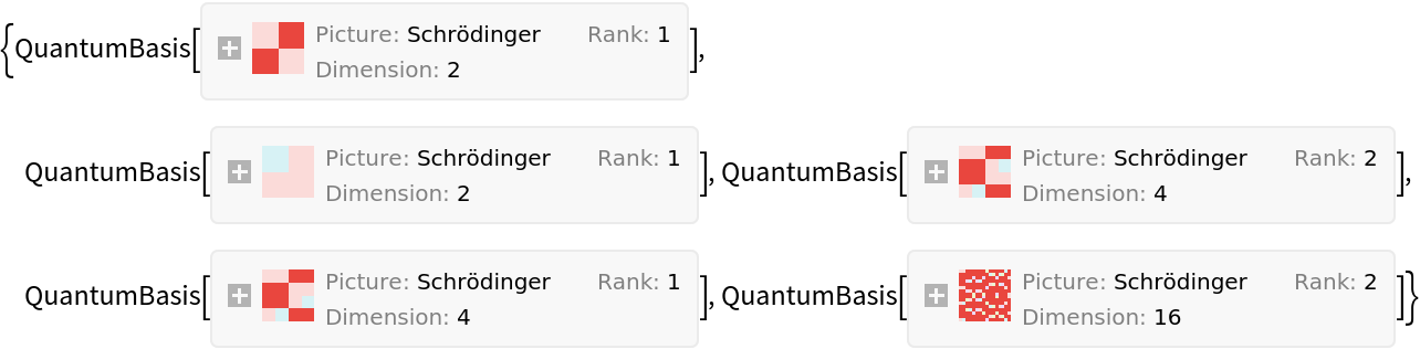
In order to use QuantumBasis, one gives dimension information as arguments, which will be interpreted as the computational basis. Alternatively, an association can be given with the basis name as the key and the corresponding basis elements as the values.
Define a 2D quantum basis (computational):
Given a basis of dimension n, the basis elements will be indexed by the key  with :
Use QuantumBasis[n,m] to define a basis for m qudits of dimension n (for which the overall dimension will be ). For example, define a 2×2×2-dimensional quantum basis (with three qubits):
Use QuantumBasis[{n1,n2,…,nm}] to define an n1×n2×n3×…×nm-dimensional Hilbert space of qudits as a list. For example, define a 3×5-dimensional quantum basis (with two qudits):
A basis can also be defined as an association with the basis element names as keys and the corresponding vectors as values:
There are many 'named' bases built into the quantum framework, including "Computational", "PauliX", "PauliY", "PauliZ", "Fourier", "Identity", "Schwinger", "Pauli", "Dirac" and "Wigner":
After a basis object has been defined, it is straightforward to construct quantum states and operators. A quantum state is represented by a QuantumState object and a quantum operator is represented by QuantumOperator.
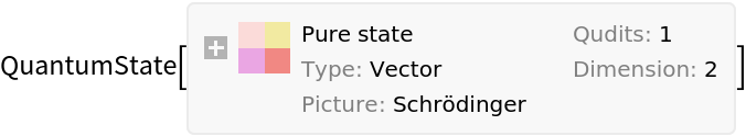
A pure quantum state is represented as a vector for which the elements are amplitudes. The corresponding basis should be given in this format: QuantumState[arg1,arg2], where arg1 specifies amplitudes or the density matrix, and arg2 specifies the basis. With no basis specified, the default basis will be the computational basis, the dimension of which depends on the amplitude vector given in arg1.
Note that the big endian convention is in use, such that qubits are labeled left-to-right, starting with 1. For example, the decimal representation of (which means ⊗⊗3) is . Additionally, for the eigenvalues of Pauli-Z, there is:
Denote the eigenstate {1,0} by (which corresponds to +1 eigenvalue), and {0,1} by (which corresponds to the eigenvalue -1).
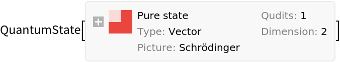
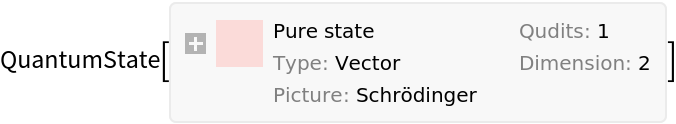
Define a pure 2-dimensional quantum state (qubit) in the Pauli-X basis:
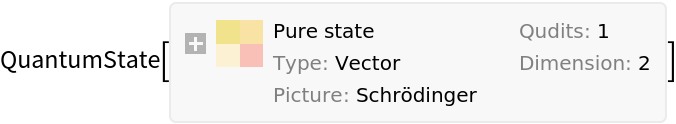
If the basis is not specified, the default is the computational basis of dimensions ( qubits):
If the vector has more than 2 elements, it is interpreted as an -qubit state, unless the dimension is specified. If fewer than 2n amplitudes are specified, right-padding is applied to reach the 2n "ceiling":
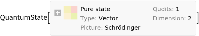
Here is the same amplitude vector, but this time with the dimension specified:
Binary strings can also be used as inputs:
Many "named" states are available through the framework:
Using associations, one can create a superposition of states, where the keys are lists of corresponding indexes and the values are amplitudes.
Create a superposition of 3 qubits (i.e. QuantumBasis[2,3] as 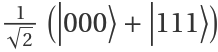 ):
):
A superposition can also be created by simply adding two quantum state objects. For example, the previous state can also be constructed as follows:
With a built-in basis specified, amplitudes correspond to the basis elements. For example, use the Bell basis:
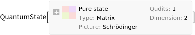
A state can also be defined by inputting a density matrix:
For pure states, one can get the corresponding normalized state vector:
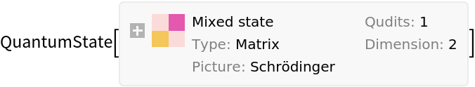
Define a generic Bloch vector:
Test to see if it is a mixed state:
Calculate its von Neumann entropy:
Compute its purity:
Note that one can directly use a Bloch vector as an input:
Test to see if a matrix is positive semidefinite:
A matrix that is not positive semidefinite cannot be a density matrix in standard quantum mechanics (with some exceptional cases, such as ZX formalism). Here is the result when it is attempted to define a state using such a matrix:
When a matrix is given as input but no basis is given, the default basis will be computational:
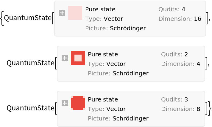
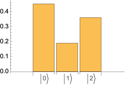
Using , define a quantum state in a 2×4-dimensional basis (and note the number of qudits):
Define a quantum state in 8D Hilbert space (with one 8-dimensional qudit only):
One can also define a state in a given basis and then transform it into a new basis. For example, transform  , the computational basis, into the Pauli-X basis {,}:
Return the amplitudes:
Note that the states are the same, but defined in different bases:
One can use QuantumTensorProduct to construct different states or operators. Create a tensor product of a + state with three qubits  :
:
Another way of defining  is to first define a basis and then assign amplitudes:
Quantum Operators (10)
Quantum operators can be defined by a matrix or by specifying eigenvalues with respect to a QuantumBasis. Additionally, there are many built-in named operators that can be used.
Define a Pauli-X operator:
Apply a Pauli-X operator to a symbolic state  :
:
Test to see if the application of the Pauli-X operator yields the correct state:
Apply the Hadamard operator  :
:
Test to see if the application of the Hadamard operator yields the correct state:
One can also compose operators. Here is a composition of two Hadamard operators and one Pauli-Z operator:
Check the relation σx=HσxH:
Multi-qubit operators can take specific orders.
For instance, first define the state α+β:
Then, apply a Pauli-X operator on the second qubit only (by defining an order for the operator):
Test the result:
For multi-qudit cases, one can define an order or construct the operator using QuantumTensorProduct. For example:
Generalize Pauli matrices to higher dimensions:
Convert to matrix form:
Generalize the Hadamard operator to more qubits:
Test that the Hadamard operator can be constructed as a tensor product:
One can define a "Controlled" operator with specific target and control qudits:
Return the control and target qudits:
Get the action of the operator (T-controlled (1, 2)) on :
Note that "CT" is also a "named" controlled operator in this framework:
One can create a new operator by performing some mathematical operations (e.g., exponential, fraction power, etc.) on a quantum operator:
Show that the result is the same as a rotation operator around x:
Get the fractional power of the NOT operator:
Quantum Measurement (12)
In the Wolfram Quantum Framework, one can study projective measurements or, generally, any positive operator-valued measurement (POVM) using QuantumMeasurementOperator.
PVMs (projective measurements) (5)
A measurement can be defined by specifying the corresponding measurement basis.
Measure a 3D system in its state basis:
Test to confirm that the measured states are the same as the basis states:
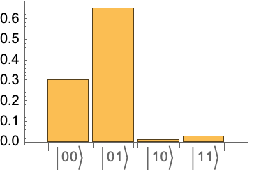
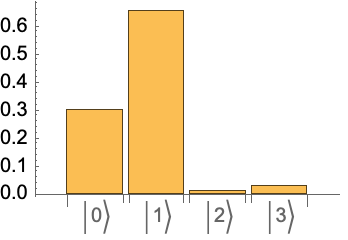
Measure a 2-qubit system in the computational basis:
Note the labels for the corresponding eigenvalues, from 0 to n-1 as follows:
For composite systems, one can measure one or more qudits. This can be done by specifying an order for QuantumMeasurementOperator.
2D×3D composite system:
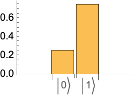
Measure only the first qudit:
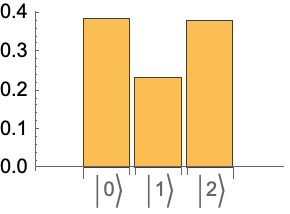
Measure only the second qudit:
Measure both qudits:
One can use the following format for "named" bases and their corresponding eigenvalues: QuantumMeasurementOperator[name→eigenvalues].
For example, define a measurement operator with a "named" QuantumBasis (as an eigenbasis) and a list of eigenvalues:
POVMs (7)
One can also give a list of POVM elements by which to define the measurement operator:
Check that all POVM elements are explicitly positive semidefinite:
Check the completeness relations:
Measure POVMs on a quantum state:
Get the post-measurement states:
Get the corresponding probabilities:
Show that post-measurement states are the same as states initially defined as POVMs:
Quantum Partial Tracing, Distance and Entanglement (4)
In the framework, there are some functionalities to explore the quantum distance, entanglement monotones and partial tracing, as well as other useful features.
Trace out the second subsystem in a 2-qubit state:
A partial trace can also be applied to QuantumBasis:
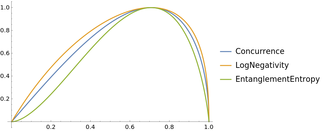
There are several metrics by which one can measure entanglement between two qudits, such as concurrence, entanglement entropy, negativity, etc. The calculation of entanglement measure is represented by the QuantumEntanglementMonotone function.
Plot various entanglement measures for the state  :
:
To know whether a state is entangled or separable without computing its measure, use QuantumEntangledQ.
Check whether subsystems 1 and 3 are entangled in the "W" state:
In quantum information, there exist notions of distance between quantum states, such as fidelity, trace distance, Bures angle, etc. One can use QuantumDistance to compute the distance between two quantum states with various metrics.
Measure the trace distance between a pure state and a mixed state:
Quantum Circuits (4)
One may create a list of QuantumOperator and/or QuantumMeasurementOperator objects to build a quantum circuit, which can be represented as a QuantumCircuitOperator object.
Construct a quantum circuit that includes a controlled Hadamard gate:
The wire labels can be customized:
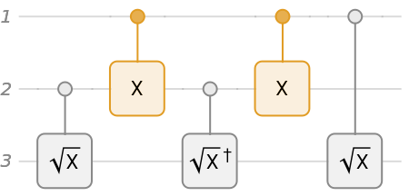
Construct a Toffoli gate as a circuit:
Show that the circuit is the same as the Toffoli gate:
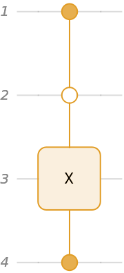
Define a combination of control-0 and control-1 qubits:
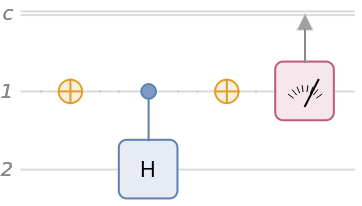
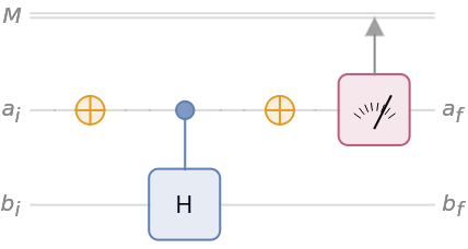
Measurement operators can also be added to a quantum circuit. For a single-qubit unitary operator with eigenvalues ±1, a measurement of can be implemented in the following circuit (note that here, Pauli-Y is considered a operator):
Applying the circuit operators to a quantum state results in a quantum measurement:
Calculate the state of the second qubit after the measurement by tracing over the first qubit:
The post-measurement states of the second qubit should be the same as the Pauli-Y eigenstates.
Superdense coding (5)
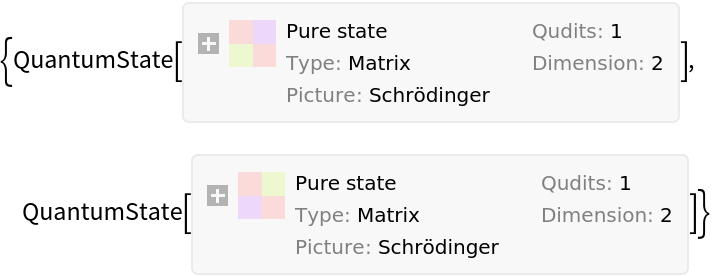
Alice wants to send Bob two classical bits: 00, 01, 10 or 11. She can do so by using a single qubit if her qubit and Bob's are initially prepared as Bell states:
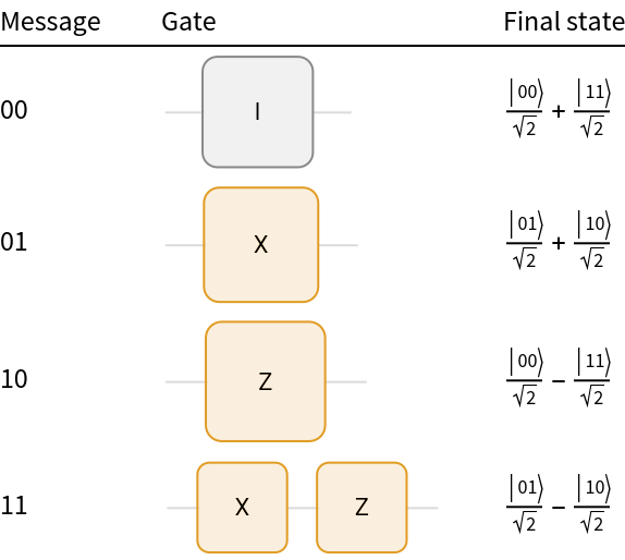
Depending on Alice's intended message, she will perform the following operations on her qubit:
1. To send 00, she does nothing.
2. To send 01, she applies the X-gate.
3. To send 10, she applies the Z-gate.
4. To send 11, she applies the X-gate and then the Z-gate.
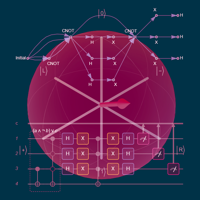
Such operations can be represented as circuits, each with a final state resulting from application of its respective gate(s) to the initial Bell state:
Next, Alice sends her qubit to Bob through a quantum channel. If Bob performs a Bell measurement on his qubits, he receives Alice's message.
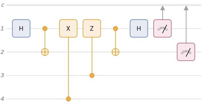
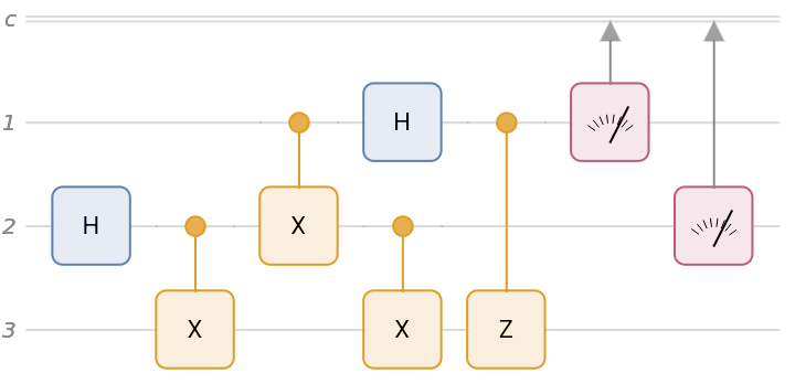
Alice's "messaging" with Bob can be fully implemented in a quantum circuit using two ancillary qubits. In the circuit, the first qubit is Alice's, the second one is Bob's and the third and the fourth are the ancillary qubits. Note that Alice sends her qubit to Bob and Bob performs a measurement on qubits 1 and 2:
Define an initial state as , where is the code that Alice wants to send Bob, which is encoded in two ancillary qubits (qubits 3 and 4).
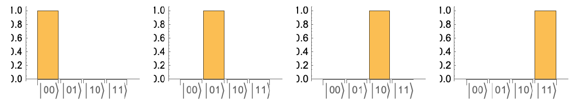
Run the state through the circuit and return the outcome probabilities:
For each case, Bob finds Alice's code with probability 1.
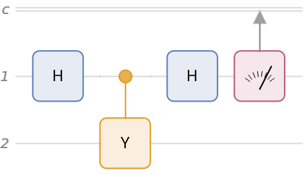
Quantum teleportation (4)
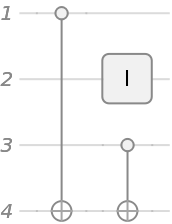
Quantum teleportation is the reverse of superdense coding. Here, one wants to teleport a generic unknown quantum bit. Suppose that Alice wants to send a qubit (qubit 1) to Bob. To implement a quantum circuit for teleporting a qubit, Alice and Bob share an entangled state (qubits 2 and 3). Qubits 1 and 2 represent Alice's system, while qubit 3 is Bob's. The goal is to transfer the state of Alice's first qubit to Bob's qubit.
Set up a circuit:
The state to be teleported is =α+β, where α and β are unknown amplitudes. The input state of the circuit is as follows:
Given the result of Alice's measurement on the first and second qubits, get the post-measurement states:
Regardless of measurement results, the state of the third qubit is the same state as the original first qubit =α+β (with only a normalization difference). Trace out the first and second qubits and compare the reduced state of qubit 3 only:
Bernstein–Vazirani algorithm (3)
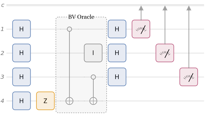
The goal of the Bernstein–Vazirani algorithm is to find a secret string bit as s using the action of a Bernstein–Vazirani oracle (i.e. which should be treated as a black box), which is defined by this transformation: → with the index register state of n-qubits, and the state of an ancillary qubit carrying the result.
A Bernstein–Vazirani oracle for the secret bit of 101:
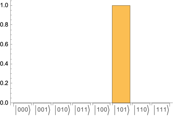
A Bernstein–Vazirani circuit for the secret bit of 101:
As expected, the only measurement outcome corresponds to the secret bit string:
Grover's search algorithm (14)
The goal of Grover's search algorithm is to find the solutions of a Boolean function . This can be done using the named circuits or oracles in the quantum framework.
The action of a Boolean oracle is defined by this transformation: → with the index register state of n-qubits, and the state of an ancillary qubit carrying the result of the Boolean function f(x); meaning if =, then it will be if x is a solution of f(x), and unchanged if it is not.
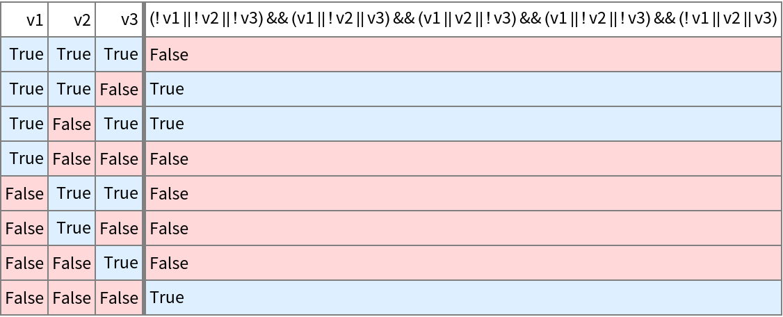
Define a Boolean function of 3-SAT with five clauses:
Here is the truth table for this Boolean function:
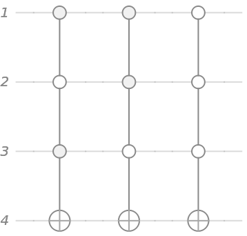
The corresponding oracle's quantum circuit:
The diagram of the oracle:
Prepare the 4-qubit in the previous circuit (i.e. the ancillary qubit) as a 0-state, and then other qubits (1–3) in the index register states. To compare with the truth table, create the index register states |x> in the order |2n-1> down to |0:
Create a list with elements {|x>,|q⊕f(x)}:
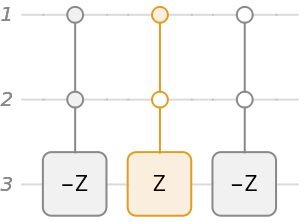
The action of a phase oracle can be defined as the following transformation: with the index register state of n-qubits:
The diagram of the oracle:
Create a list with elements {|x>,(-1)f(x)|x>}:
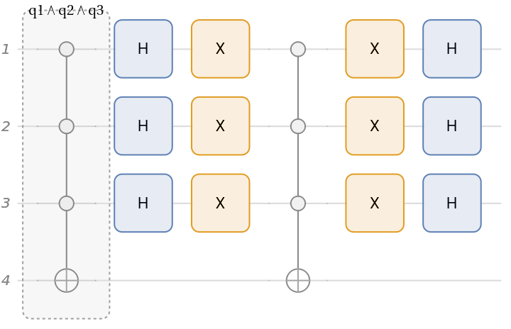
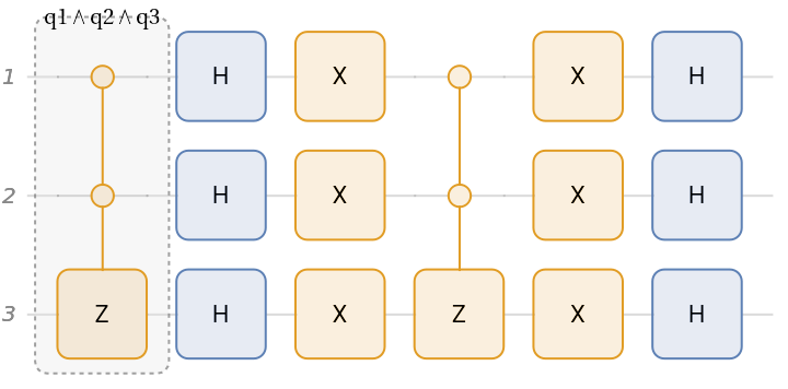
Generate the corresponding Grover circuit using a Boolean oracle:
Generate a Grover circuit using the phase oracle for a Boolean function:
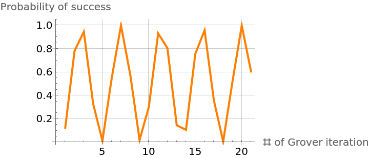
Given a Grover phase circuit for a Boolean function, calculate the probability of success of the algorithm:
Calculate the success probability after each iteration (note 111 is the solution of the Boolean function):
Plot the success probability:
As expected, this follows the formula for the probability of success 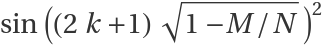 , where M is the number of correct solutions out of a total N after k steps
Quantum phase estimation (5)
The quantum phase estimation algorithm solves the problem of finding in the eigenvalue equation = , where is a unitary operator. The inputs of the algorithm are qubits at the initial state  . The output is
  .
Consider a phase shift as the unitary operator in which the aim is to find the phase θ:
.
Consider a phase shift as the unitary operator in which the aim is to find the phase θ:
To specify the corresponding quantum circuit, one can use the built-in circuit "PhaseEstimation" that takes two input arguments: a unitary operator U and an integer n. The integer n specifies the number of qubits and controlled-Uj operators in the circuit, with j=0,1,…,n-1. The accuracy of phase estimation and the success probability depends on n:
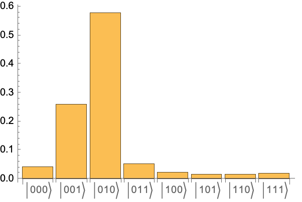
Return the corresponding measurement, with all qubits prepared in state:
Given the outcome with the largest probability, estimate the phase:
As expected, it is a rough estimate, since a small value was chosen for n. If one increases n, with a higher probability, one can get a better estimate of the phase.
Estimate the phase (the expected value is 1/5=0.2) for n=6:


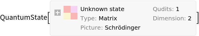
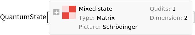
![m = RandomComplex[{-1 - I, 1 + I}, {8, 8}];
\[Rho] = ConjugateTranspose[m] . m;
state = QuantumState[\[Rho]]](https://www.wolframcloud.com/obj/resourcesystem/images/b7a/b7acdc31-f5bd-43d2-a50f-580e75215231/1-0-31/1610538aa74fc9c5.png)


![\[Psi]1 = QuantumTensorProduct[QuantumState["Plus"], QuantumState["Plus"], QuantumState["Plus"]];
\[Psi]1["Formula"]](https://www.wolframcloud.com/obj/resourcesystem/images/b7a/b7acdc31-f5bd-43d2-a50f-580e75215231/1-0-31/629a380b45a6293f.png)


![QuantumOperator[{"Hadamard", 3}] == QuantumTensorProduct[QuantumOperator["H"], QuantumOperator["H"], QuantumOperator["H"]]](https://www.wolframcloud.com/obj/resourcesystem/images/b7a/b7acdc31-f5bd-43d2-a50f-580e75215231/1-0-31/27bf769838b5874b.png)


![hamiltonian = QuantumOperator[
Subscript[\[Omega], 1]/2 Cos[\[Alpha]] QuantumOperator["Z"] + Subscript[\[Omega], 1]/
2 Sin[\[Alpha]] (Cos[\[Omega] t] QuantumOperator["X"] + Sin[\[Omega] t] QuantumOperator["Y"]), "ParameterSpec" -> t];](https://www.wolframcloud.com/obj/resourcesystem/images/b7a/b7acdc31-f5bd-43d2-a50f-580e75215231/1-0-31/11e1869f5e16ba15.png)


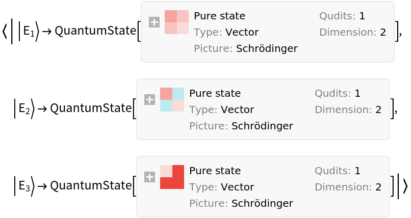
![states = {QuantumState[-(1/2) {1, Sqrt[3]}], QuantumState[-(1/2) {1, -Sqrt[3]}], QuantumState["0"]};
{e1, e2, e3} = 2/3 QuantumOperator[#[#["Dagger"]]] & /@ states;
povm = {e1, e2, e3};](https://www.wolframcloud.com/obj/resourcesystem/images/b7a/b7acdc31-f5bd-43d2-a50f-580e75215231/1-0-31/329a5fd2d0e0e344.png)
![Plot[{QuantumEntanglementMonotone[
QuantumState[{\[Alpha], 0, 0, Sqrt[1 - \[Alpha]^2]}], {{1}, {2}}, "Concurrence"], QuantumEntanglementMonotone[
QuantumState[{\[Alpha], 0, 0, Sqrt[1 - \[Alpha]^2]}], {{1}, {2}}, "LogNegativity"], QuantumEntanglementMonotone[
QuantumState[{\[Alpha], 0, 0, Sqrt[1 - \[Alpha]^2]}], {{1}, {2}}, "EntanglementEntropy"]}, {\[Alpha], 0, 1}, PlotLegends -> {"Concurrence", "LogNegativity", "EntanglementEntropy"}]](https://www.wolframcloud.com/obj/resourcesystem/images/b7a/b7acdc31-f5bd-43d2-a50f-580e75215231/1-0-31/7a14621748193a7f.png)
![qc["Diagram", "WireLabels" -> {{Placed["\!\(\*SubscriptBox[\(a\), \(i\)]\)", Left],
Placed["\!\(\*SubscriptBox[\(a\), \(f\)]\)", Right]}, {Placed[
"\!\(\*SubscriptBox[\(b\), \(i\)]\)", Left], Placed["\!\(\*SubscriptBox[\(b\), \(f\)]\)", Right]}}, "MeasurementWireLabel" -> "M"]](https://www.wolframcloud.com/obj/resourcesystem/images/b7a/b7acdc31-f5bd-43d2-a50f-580e75215231/1-0-31/57b1de4cca33cd84.png)
![qc = QuantumCircuitOperator[{{"C", Sqrt["X"]} -> {2, 3}, "CX", {"C", Sqrt[QuantumOperator["X"]]["Dagger"]} -> {2, 3}, "CX" -> {1, 2}, {"C", Sqrt["X"]} -> {1, 3}}]; qc["Diagram"]](https://www.wolframcloud.com/obj/resourcesystem/images/b7a/b7acdc31-f5bd-43d2-a50f-580e75215231/1-0-31/00f8198d1c943b59.png)
![TableForm[{#1, QuantumCircuitOperator[#2]["Diagram", "WireLabels" -> None], QuantumCircuitOperator[{#2, QuantumOperator["Identity", {2}]}][
QuantumState["PhiPlus"]]["Formula"]} & @@@ {{"00", QuantumOperator["Identity"]}, {"01", QuantumOperator["X"]}, {"10",
QuantumOperator["Z"]}, {"11", {QuantumOperator["X"], QuantumOperator["Z"]}}}, TableHeadings -> {None, {"Message", "Gate", "Final state"}}]](https://www.wolframcloud.com/obj/resourcesystem/images/b7a/b7acdc31-f5bd-43d2-a50f-580e75215231/1-0-31/25f653bb0e30faa9.png)
![superdense = QuantumCircuitOperator[{"H", "CNOT", "CX" -> {4, 1}, "CZ" -> {3, 1},
"CNOT", "H", {1}, {2}}];
superdense["Diagram"]](https://www.wolframcloud.com/obj/resourcesystem/images/b7a/b7acdc31-f5bd-43d2-a50f-580e75215231/1-0-31/5edfa9a0eaf8bd8f.png)
![TableForm[
Transpose[{Table[
QuantumState[{"Register", 3, i}]["Formula"], {i, 2^3 - 1, 0, -1}],
QuantumPartialTrace[oracle[#], {1, 2, 3}]["Formula"] & /@ states}], TableHeadings -> {None, {"|x>", "|q\[CirclePlus]f(x)>"}}]](https://www.wolframcloud.com/obj/resourcesystem/images/b7a/b7acdc31-f5bd-43d2-a50f-580e75215231/1-0-31/0c1af927616dcd7f.png)

![Module[{index = Table[QuantumState[{"Register", 3, i}], {i, 2^3 - 1, 0, -1}]},
TableForm[
Transpose[{#["Formula"] & /@ index, phaseOracle[#]["Formula"] & /@ index}], TableHeadings -> {None, {"|x>", "(-1\!\(\*SuperscriptBox[\()\), \(f \((x)\)\)]\)|x>"}}]]](https://www.wolframcloud.com/obj/resourcesystem/images/b7a/b7acdc31-f5bd-43d2-a50f-580e75215231/1-0-31/7857720edd685729.png)

![circuit = QuantumCircuitOperator[{"PhaseEstimation", QuantumOperator[{"Phase", 2 Pi phase}], n}];
circuit["Diagram", FontSize -> 11]](https://www.wolframcloud.com/obj/resourcesystem/images/b7a/b7acdc31-f5bd-43d2-a50f-580e75215231/1-0-31/10f038e4c0acb826.png)

![With[{m = QuantumCircuitOperator[{"PhaseEstimation", N@QuantumOperator[{"Phase", 2 Pi phase}], 6}][]}, FromDigits[Keys[TakeLargest[m["Probabilities"], 1]][[1]]["Name"], 2]/
2^6 // N]](https://www.wolframcloud.com/obj/resourcesystem/images/b7a/b7acdc31-f5bd-43d2-a50f-580e75215231/1-0-31/169adc1b8f47a77b.png)