Wolfram Language Paclet Repository

Community-contributed installable additions to the Wolfram Language

Primary Navigation

    • Cloud & Deployment
    • Core Language & Structure
    • Data Manipulation & Analysis
    • Engineering Data & Computation
    • External Interfaces & Connections
    • Financial Data & Computation
    • Geographic Data & Computation
    • Geometry
    • Graphs & Networks
    • Higher Mathematical Computation
    • Images
    • Knowledge Representation & Natural Language
    • Machine Learning
    • Notebook Documents & Presentation
    • Scientific and Medical Data & Computation
    • Social, Cultural & Linguistic Data
    • Strings & Text
    • Symbolic & Numeric Computation
    • System Operation & Setup
    • Time-Related Computation
    • User Interface Construction
    • Visualization & Graphics
    • Random Paclet
    • Alphabetical List
  • Using Paclets
    • Get Started
    • Download Definition Notebook
  • Learn More about Wolfram Language

QuantumFramework

Tutorials

  • Getting Started
  • Quantum Machine Learning in Phase Space
  • Quantum Object Composition
  • Time Evolution

Guides

  • Wolfram Quantum Computation Framework

Tech Notes

  • Bell's Theorem: CHSH inequality
  • Circuit Diagram
  • Exploring Fundamentals of Quantum Theory
  • An IBM Quantum Error Map
  • QPU Service Connection
  • Quantum object abstraction
  • Quantum Optimization
  • Second Quantization Functions
  • Sending Queries to IBM QPUs
  • Tensor Network
  • Quantum Computation

Symbols

  • CliffordChannel
  • EinsteinSummation
  • GraphState
  • IBMJob
  • IBMJobSubmit
  • LocalComplement
  • PauliStabilizer
  • QiskitCircuit
  • QiskitTarget
  • QuantumBasis
  • QuantumChannel
  • QuantumCircuitMultiwayGraph [EXPERIMENTAL]
  • QuantumCircuitOperator
  • QuantumDistance
  • QuantumEntangledQ
  • QuantumEntanglementMonotone
  • QuantumEvolve
  • QuantumMeasurement
  • QuantumMeasurementOperator
  • QuantumMeasurementSimulation
  • QuantumMPS [EXPERIMENTAL]
  • QuantumOperator
  • QuantumPartialTrace
  • QuantumPhaseSpaceTransform
  • QuantumQASM
  • QuantumShortcut [EXPERIMENTAL]
  • QuantumSimilarity
  • QuantumStateEstimate [EXPERIMENTAL]
  • QuantumState
  • QuantumTensorProduct
  • QuantumWignerMICTransform [EXPERIMENTAL]
  • QuantumWignerTransform [EXPERIMENTAL]
  • QuditBasis
  • QuditName
  • StabilizerFrame
  • StabilizerStateQ

Quantum Machine Learning in Phase Space

A quantum circuit is a tensor network, and a tensor network contraction is a sequence of array products - the computation a neural net performs. The framework closes that loop: a
QuantumCircuitOperator
compiles to a tensor network, and
Wolfram`TensorNetworks`
contracts that network into a
NetGraph
rather than an array, with every circuit tensor held in a
NetArrayLayer
. The circuit becomes the model. Nothing about the forward computation is assembled by hand; the only layer added here is the loss.
The net framework computes over real numbers, and that is not an obstacle: in the phase-space picture a state is a Wigner quasi-probability vector and every circuit tensor is real, so the whole pipeline stays inside what a net can represent. This tutorial compiles a circuit to a net, differentiates through it, and trains a gate until gradient descent recovers a rotation angle.
In[1]:=
<<Wolfram`QuantumFramework`

A Circuit Is the Model

A circuit can carry its own initial state, so the whole computation - prepare, then rotate - is one object:
In[2]:=
qc=
QuantumCircuitOperator

QuantumState
["0"],"RY"[0.7]
Out[2]=
QuantumCircuitOperator
​

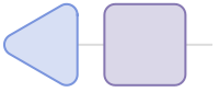
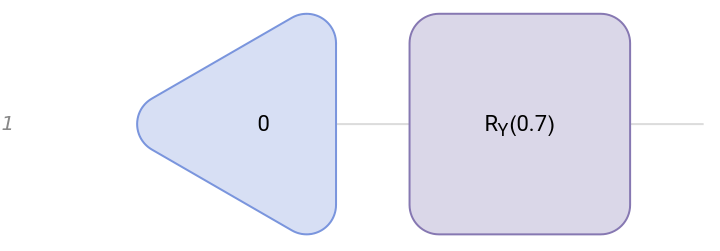
Its diagram shows the state feeding the gate:
In[3]:=
qc["Diagram"]
Out[3]=
QuantumPhaseSpaceTransform
moves it to the phase-space picture, where each qubit's 2-dimensional Hilbert space becomes a 4-dimensional space of Wigner components:
In[4]:=
ps=
QuantumPhaseSpaceTransform
[qc]
Out[4]=
QuantumCircuitOperator
​


The Circuit as a Tensor Network

The
"TensorNetwork"
property compiles the circuit into a network of one tensor per element.
"Computational"->False
keeps the tensors in the phase-space frame, where they are real; without it, basis-change tensors in the computational frame enter and are complex:
In[5]:=
tn=ps["TensorNetwork","Computational"False]
Out[5]=
TensorNetwork
Tensors: 2
Binary: Yes
Free indices: 1
Sparse: Yes
Output dimension: 4
​

The largest imaginary part across every entry of every tensor is exactly zero:
In[6]:=
Max[Max[Abs[Im[N[Flatten[Normal[#]]]]]]&/@TensorNetworkTensors[tn]]
Out[6]=
0
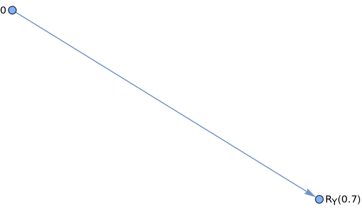
The network is a graph, with the state and the gate as its two nodes:
In[7]:=
ps["TensorNetworkGraph","Computational"False]
AllowKernelInitialization::shdw:SymbolAllowKernelInitializationappearsinmultiplecontexts{System`,Global`};definitionsincontextSystem`mayshadoworbeshadowedbyotherdefinitions.
Out[7]=

Contracting to a Net

Wolfram`TensorNetworks`
chooses the pairwise contraction order:
In[8]:=
path=GreedyContractionPath[tn]
Out[8]=
{{1,2}}
TensorNetworkContraction
with
Method->"NetGraph"
performs the same contraction, but instead of computing the array it wires the computation as a net: each leaf tensor becomes a
NetArrayLayer
, and each pairwise contraction becomes reshape, transpose and dot layers:
In[9]:=
net=TensorNetworkContraction[tn,path,Method"NetGraph"]
Out[9]=
NetGraph
Number of inputs:
0
Outputport:
vector(size: 4)

The net takes no input and its output is the state the circuit produces, so running it gives the Wigner vector directly - no separate state extraction:
In[10]:=
net[]
Out[10]=
{0.25,0.161054,0.191211,0.}
That is the Wigner vector of the state an RY rotation by 0.7 produces from the initial one:
In[11]:=
ChopNormalN
QuantumPhaseSpaceTransform

QuantumState
[{Cos[0.35],Sin[0.35]}]["StateVector"]
Out[11]=
{0.25,0.161054,0.191211,0}
Because the net is a source net, it is also an array container: its shape reads off the output port with nothing evaluated:
In[12]:=
ArrayDimensions[net]
Out[12]=
{4}

The Gate as a Trainable Parameter

To train a gate rather than a state, compile the gate alone. With
"PrependInitial"->False
no initial state is attached, and the net's output is the gate's own phase-space kernel:
In[13]:=
gate[theta_]:=Blockp=
QuantumPhaseSpaceTransform

QuantumCircuitOperator
[{"RY"[theta]}],t,​​t=p["TensorNetwork","Computational"False,"PrependInitial"False];​​TensorNetworkContraction[t,GreedyContractionPath[t],Method"NetGraph"];​​gate[0.7][]
Out[13]=
{{1.,0.,0.,0.},{0.,0.764842,0.644218,0.},{0.,-0.644218,0.764842,0.},{0.,0.,0.,1.}}
The kernel is a rotation by the angle in its middle block, so the angle can be read straight off it:
In[14]:=
ArcTan@@Chop[gate[0.7][]]〚2,{2,3}〛
Out[14]=
0.7

Learning the Angle

Take the circuit at 0.7 as the target and a circuit at 0 as the model. The only thing built by hand is the loss: the compiled circuit becomes one node of a net whose other node is a
MeanAbsoluteLossLayer
.
In[15]:=
target=gate[0.7][];​​lossNet=NetGraph["circuit"gate[0.],"loss"MeanAbsoluteLossLayer[],​​{"circuit"NetPort["loss","Input"],NetPort["Target"]NetPort["loss","Target"]}]
Out[15]=
NetGraph
Targetport:
matrix(size: 4×4)
Lossport:
real

Compiling the circuit made the gate a learnable parameter of the net. It is the only one:
In[16]:=
Keys[Information[lossNet,"Arrays"]]
Out[16]=
{{circuit,tensor,Array}}
The target enters through an input port, and the loss comes out of an output port, which is all
NetTrain
needs:
In[17]:=
Information[lossNet,"InputPorts"]
Out[17]=
Target{4,4}
The model starts at the identity, an angle of zero:
In[18]:=
ArcTan@@Chop[Normal[NetExtract[lossNet,{"circuit","tensor","Array"}]]]〚2,{2,3}〛
Out[18]=
0.
In[19]:=
lossNet["Target"target]
Out[19]=
0.109922
Training is then ordinary
NetTrain
: one example, the net's own
"Loss"
port as the objective, and the gate array is what gets updated.
In[20]:=
trained=NetTrain[lossNet,"Target"{target},LossFunction"Loss",​​MaxTrainingRounds2000,TrainingProgressReportingNone];​​trained["Target"target]
Out[20]=
0.0000529364
Training through the compiled circuit recovered the rotation angle:
In[21]:=
ArcTan@@Chop[Normal[NetExtract[trained,{"circuit","tensor","Array"}]]]〚2,{2,3}〛
Out[21]=
0.700006

Details

Possible Issues

Training a gate against a single input state does not determine it. The gate above is trained against its whole kernel, which pins every column; fitting only the circuit's output vector would leave the gate's action on the rest of the space free, and the recovered angle would mean nothing.

© 2026 Wolfram. All rights reserved.

  • Legal & Privacy Policy
  • Contact Us
  • WolframAlpha.com
  • WolframCloud.com