Wolfram Language Paclet Repository

Community-contributed installable additions to the Wolfram Language

Primary Navigation

    • Cloud & Deployment
    • Core Language & Structure
    • Data Manipulation & Analysis
    • Engineering Data & Computation
    • External Interfaces & Connections
    • Financial Data & Computation
    • Geographic Data & Computation
    • Geometry
    • Graphs & Networks
    • Higher Mathematical Computation
    • Images
    • Knowledge Representation & Natural Language
    • Machine Learning
    • Notebook Documents & Presentation
    • Scientific and Medical Data & Computation
    • Social, Cultural & Linguistic Data
    • Strings & Text
    • Symbolic & Numeric Computation
    • System Operation & Setup
    • Time-Related Computation
    • User Interface Construction
    • Visualization & Graphics
    • Random Paclet
    • Alphabetical List
  • Using Paclets
    • Get Started
    • Download Definition Notebook
  • Learn More about Wolfram Language

QuantumFramework

Tutorials

  • Getting Started
  • Quantum Machine Learning in Phase Space
  • Quantum Object Composition
  • Time Evolution

Guides

  • Wolfram Quantum Computation Framework

Tech Notes

  • Bell's Theorem: CHSH inequality
  • Circuit Diagram
  • Exploring Fundamentals of Quantum Theory
  • An IBM Quantum Error Map
  • QPU Service Connection
  • Quantum object abstraction
  • Quantum Optimization
  • Second Quantization Functions
  • Sending Queries to IBM QPUs
  • Tensor Network
  • Quantum Computation

Symbols

  • CliffordChannel
  • EinsteinSummation
  • GraphState
  • IBMJob
  • IBMJobSubmit
  • LocalComplement
  • PauliStabilizer
  • QiskitCircuit
  • QiskitTarget
  • QuantumBasis
  • QuantumChannel
  • QuantumCircuitMultiwayGraph [EXPERIMENTAL]
  • QuantumCircuitOperator
  • QuantumDistance
  • QuantumEntangledQ
  • QuantumEntanglementMonotone
  • QuantumEvolve
  • QuantumMeasurement
  • QuantumMeasurementOperator
  • QuantumMeasurementSimulation
  • QuantumMPS [EXPERIMENTAL]
  • QuantumOperator
  • QuantumPartialTrace
  • QuantumPhaseSpaceTransform
  • QuantumQASM
  • QuantumShortcut [EXPERIMENTAL]
  • QuantumSimilarity
  • QuantumStateEstimate [EXPERIMENTAL]
  • QuantumState
  • QuantumTensorProduct
  • QuantumWignerMICTransform [EXPERIMENTAL]
  • QuantumWignerTransform [EXPERIMENTAL]
  • QuditBasis
  • QuditName
  • StabilizerFrame
  • StabilizerStateQ

Time Evolution

QuantumEvolve
solves the equation of motion of a quantum system. Which equation that is depends on what you hand it: the Schrodinger equation for a closed system, the Lindblad master equation once jump operators are present, the Heisenberg equation when the thing being evolved is an operator, and the Kossakowski equation when the jump operators are correlated.
The call is the same shape in every case - a Hamiltonian, optionally some dissipation, an initial condition, and a time - and the result is always an object that depends on time. Supply a time to it and you get an ordinary state or operator back, which answers every property the framework knows about.
Two choices control everything else. A bare symbol for the time solves the equation exactly, through
DSolve
; a
{t,t0,t1}
interval solves it numerically, through
NDSolve
. And an initial condition of
None
evolves the propagator instead of any particular state, which can then be applied to whatever state you like.
In[1]:=
<<Wolfram`QuantumFramework`

A Driven Qubit

A
PauliX
Hamiltonian drives a qubit between
|0〉
and
|1〉
. Evolving
|0〉
over one full period:
In[2]:=
psi=
QuantumEvolve

QuantumOperator
["PauliX"],
QuantumState
["0"],{t,0,2Pi}
Out[2]=
QuantumState
Pure state
Qudits: 1
Type: Vector
Dimension: 2

The result is a state as a function of time, and
t
is recorded on it as a parameter:
In[3]:=
psi["Parameters"]
Out[3]=
{t}
Supplying a time gives the state at that time - an ordinary
QuantumState
with nothing left symbolic:
In[4]:=
psi[1.]
Out[4]=
QuantumState
Pure state
Qudits: 1
Type: Vector
Dimension: 2

From there every state property is available as usual:
In[5]:=
psi[1.]["ProbabilitiesList"]
Out[5]=
{0.291927,0.708073}
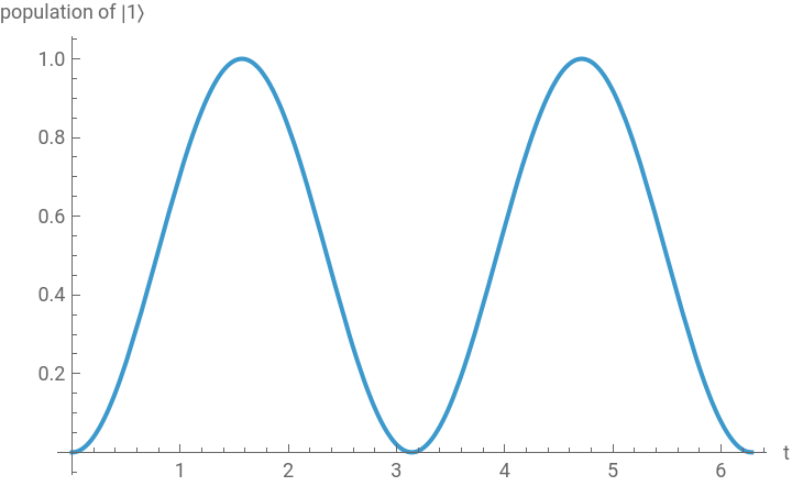
Sampling the interval shows the population sloshing between the two levels and back:
In[6]:=
Table[Round[psi[t]["ProbabilitiesList"],0.0001],{t,0,3}]
Out[6]=
{{1.,0.},{0.2919,0.7081},{0.1732,0.8268},{0.9801,0.0199}}
Plotting it gives the Rabi oscillation:
In[7]:=
Plot[psi[t]["ProbabilitiesList"]〚2〛,{t,0,2Pi},​​AxesLabel{"t","population of |1〉"}]
Out[7]=

What the Solution Actually Is

A numerically evolved state is not a table of samples and it is not a symbolic expression. Its amplitudes are the solver's own
InterpolatingFunction
, held as the state's array and applied to the time parameter:
In[8]:=
psi["State"]
Out[8]=
InterpolatingFunction
Domain: {{0.,6.28}}
Output dimensions: {2}
[t]
That single object carries the whole two-component solution, so the state still knows its own shape without interpolating anything:
In[9]:=
psi["Dimensions"]
Out[9]=
{2}
Nothing is computed until a time is supplied;
psi[1.]
is what triggers an interpolation. This matters for large systems, where the alternative - one scalar interpolation per amplitude, each carrying its own copy of the solver's time grid - costs a copy of that grid per dimension. Asking for it explicitly with
"Expand"->True
shows what is being avoided:
In[10]:=
expanded=
QuantumEvolve

QuantumOperator
["PauliX"],
QuantumState
["0"],{t,0,2Pi},"Expand"True;​​Normal[expanded["State"]]
Out[10]=
InterpolatingFunction
Domain: {{0.,6.28}}
Output: scalar
[t],InterpolatingFunction
Domain: {{0.,6.28}}
Output: scalar
[t]
The two forms give the same numbers:
In[11]:=
expanded[1.]["ProbabilitiesList"]
Out[11]=
{0.291927,0.708073}

Exact Solutions

Passing a bare symbol instead of an interval solves the equation symbolically rather than numerically:
In[12]:=
exact=
QuantumEvolve

QuantumOperator
["PauliX"],
QuantumState
["0"],t;​​Simplify[Normal[exact["StateVector"]]]
Out[12]=
{Cos[t],-Sin[t]}
That is the textbook solution, and its populations are what the plot above traced:
In[13]:=
Simplify[exact["ProbabilitiesList"],Assumptionst∈Reals]
Out[13]=
{
2
Cos[t]
,
2
Sin[t]
}
The initial state may be symbolic too, in which case so is the answer:
In[14]:=
SimplifyNormal
QuantumEvolve

QuantumOperator
["X"],
QuantumState
[{α,β}],t["StateVector"]
Out[14]=
{αCos[t]-βSin[t],βCos[t]-αSin[t]}
Omit the initial state and the time entirely and the register state
|0〉
is used, with the formal symbol
t
as the time parameter. This is the shortest thing that says anything:
In[15]:=
QuantumEvolve

QuantumOperator
["X"]
Out[15]=
QuantumState
Pure state
Qudits: 1
Type: Vector
Dimension: 2

The numerical solution agrees with the closed form to the solver's tolerance:
In[16]:=
Max[Abs[psi[1.]["ProbabilitiesList"]-{Cos[1.]^2,Sin[1.]^2}]]
Out[16]=
2.59879×
-8
10

Time-Dependent Hamiltonians

Nothing requires the Hamiltonian to be constant. A symbol in it that matches the evolution parameter simply makes the generator time dependent. This is a spin with splitting
ω
0
driven transversally at the same frequency - a resonant drive:
In[17]:=
ω0=2Pi;​​ωp=Pi/10;​​tf=2Pi/ωp;​​driven=ω0
QuantumOperator
["JZ"]+2ωpCos[ω0t]
QuantumOperator
["JX"];
With no initial state given, the register state is used, so the Hamiltonian and the time interval are the whole call:
In[18]:=
rabi=
QuantumEvolve
[driven,{t,0,tf}]
Out[18]=
QuantumState
Pure state
Qudits: 1
Type: Vector
Dimension: 2

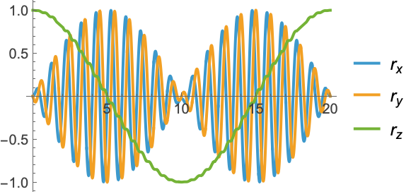
The Bloch vector traces the slow Rabi nutation underneath the fast Larmor precession. Over the interval
2π/
ω
p
it makes one full circuit from the north pole and back:
In[19]:=
Plot[Evaluate[Re[rabi[t]["BlochVector"]]],{t,0,tf},PlotRangeAll,​​PlotLegends{Subscript[r,x],Subscript[r,y],Subscript[r,z]}]
Out[19]=
Halfway through, the spin has been driven to the south pole - a
π
pulse:
In[20]:=
Round[Chop[Re[rabi[tf/2]["BlochVector"]]],0.0001]
Out[20]=
{-0.025,-0.0002,-0.9997}
The evolution is unitary throughout, so the state stays pure and the Bloch vector stays on the sphere:
In[21]:=
rabi[tf/2]["Purity"]
Out[21]=
1

Observables and Trajectories

An evolved state answers every ordinary state property once a time is given, so an observable is measured as it would be on any state:
Drawing that as a curve on the Bloch sphere shows the precession as the great circle it is:

Open Systems: the Lindblad Equation

Jump operators turn the Schrodinger equation into the Lindblad master equation,
The state is a density matrix now rather than a vector, because dissipation does not preserve purity. Purity falls from 1 toward the maximally mixed value of 1/2:
The populations equalize as it goes:

Relaxing to a Thermal State

Starting from a pure state tilted off the axis:

The Liouvillian and the Propagator

It acts on a density matrix flattened into a vector, so for a qubit its matrix is 4x4 rather than 2x2:
Because it is the map and not a trajectory, it can be applied to any state without solving again:
Solving the same problem directly as a Lindblad equation gives the same answer, to the solver's tolerance:
The propagator also exists for closed systems, where it is the familiar unitary. Solved exactly it is a closed form:

The Heisenberg Picture

In the Heisenberg picture the observable moves and the state does not:
They agree to machine precision across the interval, since both read the same solved propagator:

The Kossakowski Equation

The Lindblad equation assumes the jump operators are uncorrelated. Dropping that assumption gives the Kossakowski equation,
Two atoms decaying into a shared field is the standard example. The Hamiltonian is just their bare energies:
Each atom decays through its own lowering operator:
Evolve three initial states with one excitation between them - a product state, the singlet, and the triplet. When the Hamiltonian is already a superoperator, the initial state comes directly after it:
Count the excitations left at each time with the total-number operator:
At the end of the interval they are far apart:

Watching for Events

The crossings really are crossings - evaluating the returned solution at them gives one half back:
Shading the plot between them marks out the intervals where the qubit is mostly excited:

The Equations Themselves

Details

Possible Issues

Ask for amplitudes before supplying a time and the answer is a function of the parameter rather than numbers, which is rarely what is wanted from a numerical solve. Supply the time first:
If the exact solver cannot find a closed form, the output is the unevaluated solver call it gave up on, along with a message. Here a Rabi problem with a general detuning, which has no elementary solution:
Numbers in the Hamiltonian make the same problem solvable numerically, so the fallback when a closed form does not exist is to give the parameters values and pass an interval instead.

© 2026 Wolfram. All rights reserved.

  • Legal & Privacy Policy
  • Contact Us
  • WolframAlpha.com
  • WolframCloud.com