Wolfram Language Paclet Repository
Community-contributed installable additions to the Wolfram Language
Perform analytic and numeric quantum computations
Contributed by: Wolfram Research, Quantum Computation Framework team
The Wolfram Quantum Framework brings a broad, coherent design for quantum computation, together with a host of leading-edge capabilities and full integration into Mathematica and Wolfram Language. Starting from discrete quantum mechanics, the Framework provides a high-level symbolic representation of quantum bases, states and operators. The Framework can perform measurements and is equipped with various well-known states and operators, such as Bell states and Pauli operators. Using such simulation capabilities as a foundation, one can use the Framework to model and simulate quantum circuits and algorithms, interoperate with many external quantum platforms, and send queries to quantum processing units from a Wolfram notebook.
Within the Framework, all quantum-related functions and objects are natively integrated with Wolfram Language, providing immediate access to a wide array of tools for exploring quantum computational queries and serving as a potent resource for education in the field.
To install this paclet in your Wolfram Language environment,
evaluate this code:
PacletInstall["Wolfram/QuantumFramework"]
To load the code after installation, evaluate this code:
Needs["Wolfram`QuantumFramework`"]
The Wolfram quantum framework handles many different quantum objects, including states, operators, channels, measurements, circuits, and more. It offers specialized functions for various computations like quantum evolution, entanglement monotones, partial tracing, Wigner or Weyl transformations, stabilizer formalism, and additional capabilities. Each functionality incorporates common named operations, such as Schwinger basis, GHZ state, Fourier operator, Grover circuit, and others. Perform computations seamlessly with the Wolfram quantum framework using the standard Wolfram kernel, such as the usual evaluation of codes in Mathematica. Alternatively, leverage the framework to send jobs to quantum processing units via service connections.
Create a quantum circuit composed of Pauli-X on qubits 1 and 2, Hadamard on qubit 1, CNOT with qubit 1 as the controlled and qubit 2 as the target, rotation around the z-axis by a symbolic angle ϕ on qubit 1, rotation around the z-axis by a symbolic angle θ on qubit 2, Hadamard on qubits 1 and 2, and finally, measurement in the computational basis on qubits 1 and 2.
| In[1]:= | ![qc = InterpretationBox[FrameBox[TagBox[TooltipBox[PaneBox[GridBox[List[List[GraphicsBox[List[Thickness[0.0025`], List[FaceForm[List[RGBColor[0.9607843137254902`, 0.5058823529411764`, 0.19607843137254902`], Opacity[1.`]]], FilledCurveBox[List[List[List[0, 2, 0], List[0, 1, 0], List[0, 1, 0], List[0, 1, 0], List[0, 1, 0]], List[List[0, 2, 0], List[0, 1, 0], List[0, 1, 0], List[0, 1, 0], List[0, 1, 0]], List[List[0, 2, 0], List[0, 1, 0], List[0, 1, 0], List[0, 1, 0], List[0, 1, 0], List[0, 1, 0]], List[List[0, 2, 0], List[1, 3, 3], List[0, 1, 0], List[1, 3, 3], List[0, 1, 0], List[1, 3, 3], List[0, 1, 0], List[1, 3, 3], List[1, 3, 3], List[0, 1, 0], List[1, 3, 3], List[0, 1, 0], List[1, 3, 3]]], List[List[List[205.`, 22.863691329956055`], List[205.`, 212.31669425964355`], List[246.01799774169922`, 235.99870109558105`], List[369.0710144042969`, 307.0436840057373`], List[369.0710144042969`, 117.59068870544434`], List[205.`, 22.863691329956055`]], List[List[30.928985595703125`, 307.0436840057373`], List[153.98200225830078`, 235.99870109558105`], List[195.`, 212.31669425964355`], List[195.`, 22.863691329956055`], List[30.928985595703125`, 117.59068870544434`], List[30.928985595703125`, 307.0436840057373`]], List[List[200.`, 410.42970085144043`], List[364.0710144042969`, 315.7036876678467`], List[241.01799774169922`, 244.65868949890137`], List[200.`, 220.97669792175293`], List[158.98200225830078`, 244.65868949890137`], List[35.928985595703125`, 315.7036876678467`], List[200.`, 410.42970085144043`]], List[List[376.5710144042969`, 320.03370475769043`], List[202.5`, 420.53370475769043`], List[200.95300006866455`, 421.42667961120605`], List[199.04699993133545`, 421.42667961120605`], List[197.5`, 420.53370475769043`], List[23.428985595703125`, 320.03370475769043`], List[21.882003784179688`, 319.1406993865967`], List[20.928985595703125`, 317.4896984100342`], List[20.928985595703125`, 315.7036876678467`], List[20.928985595703125`, 114.70369529724121`], List[20.928985595703125`, 112.91769218444824`], List[21.882003784179688`, 111.26669120788574`], List[23.428985595703125`, 110.37369346618652`], List[197.5`, 9.87369155883789`], List[198.27300024032593`, 9.426692008972168`], List[199.13700008392334`, 9.203690528869629`], List[200.`, 9.203690528869629`], List[200.86299991607666`, 9.203690528869629`], List[201.72699999809265`, 9.426692008972168`], List[202.5`, 9.87369155883789`], List[376.5710144042969`, 110.37369346618652`], List[378.1179962158203`, 111.26669120788574`], List[379.0710144042969`, 112.91769218444824`], List[379.0710144042969`, 114.70369529724121`], List[379.0710144042969`, 315.7036876678467`], List[379.0710144042969`, 317.4896984100342`], List[378.1179962158203`, 319.1406993865967`], List[376.5710144042969`, 320.03370475769043`]]]]], List[FaceForm[List[RGBColor[0.5529411764705883`, 0.6745098039215687`, 0.8117647058823529`], Opacity[1.`]]], FilledCurveBox[List[List[List[0, 2, 0], List[0, 1, 0], List[0, 1, 0], List[0, 1, 0]]], List[List[List[44.92900085449219`, 282.59088134765625`], List[181.00001525878906`, 204.0298843383789`], List[181.00001525878906`, 46.90887451171875`], List[44.92900085449219`, 125.46986389160156`], List[44.92900085449219`, 282.59088134765625`]]]]], List[FaceForm[List[RGBColor[0.6627450980392157`, 0.803921568627451`, 0.5686274509803921`], Opacity[1.`]]], FilledCurveBox[List[List[List[0, 2, 0], List[0, 1, 0], List[0, 1, 0], List[0, 1, 0]]], List[List[List[355.0710144042969`, 282.59088134765625`], List[355.0710144042969`, 125.46986389160156`], List[219.`, 46.90887451171875`], List[219.`, 204.0298843383789`], List[355.0710144042969`, 282.59088134765625`]]]]], List[FaceForm[List[RGBColor[0.6901960784313725`, 0.5882352941176471`, 0.8117647058823529`], Opacity[1.`]]], FilledCurveBox[List[List[List[0, 2, 0], List[0, 1, 0], List[0, 1, 0], List[0, 1, 0]]], List[List[List[200.`, 394.0606994628906`], List[336.0710144042969`, 315.4997024536133`], List[200.`, 236.93968200683594`], List[63.928985595703125`, 315.4997024536133`], List[200.`, 394.0606994628906`]]]]]], List[Rule[BaselinePosition, Scaled[0.15`]], Rule[ImageSize, 10], Rule[ImageSize, 15]]], StyleBox[RowBox[List["QuantumCircuitOperator", " "]], Rule[ShowAutoStyles, False], Rule[ShowStringCharacters, False], Rule[FontSize, Times[0.9`, Inherited]], Rule[FontColor, GrayLevel[0.1`]]]]], Rule[GridBoxSpacings, List[Rule["Columns", List[List[0.25`]]]]]], Rule[Alignment, List[Left, Baseline]], Rule[BaselinePosition, Baseline], Rule[FrameMargins, List[List[3, 0], List[0, 0]]], Rule[BaseStyle, List[Rule[LineSpacing, List[0, 0]], Rule[LineBreakWithin, False]]]], RowBox[List["PacletSymbol", "[", RowBox[List["\"Wolfram/QuantumFramework\"", ",", "\"Wolfram`QuantumFramework`QuantumCircuitOperator\""]], "]"]], Rule[TooltipStyle, List[Rule[ShowAutoStyles, True], Rule[ShowStringCharacters, True]]]], Function[Annotation[Slot[1], Style[Defer[PacletSymbol["Wolfram/QuantumFramework", "Wolfram`QuantumFramework`QuantumCircuitOperator"]], Rule[ShowStringCharacters, True]], "Tooltip"]]], Rule[Background, RGBColor[0.968`, 0.976`, 0.984`]], Rule[BaselinePosition, Baseline], Rule[DefaultBaseStyle, List[]], Rule[FrameMargins, List[List[0, 0], List[1, 1]]], Rule[FrameStyle, RGBColor[0.831`, 0.847`, 0.85`]], Rule[RoundingRadius, 4]], PacletSymbol["Wolfram/QuantumFramework", "Wolfram`QuantumFramework`QuantumCircuitOperator"], Rule[Selectable, False], Rule[SelectWithContents, True], Rule[BoxID, "PacletSymbolBox"]][{"X" -> {1, 2}, "H", "CNOT", "RZ"[\[Phi]], "RZ"[\[Theta]] -> 2, "H" -> {1, 2}, {1}, {2}}];
qc["Diagram"]](https://www.wolframcloud.com/obj/resourcesystem/images/b7a/b7acdc31-f5bd-43d2-a50f-580e75215231/0fb6073716c49ebf.png) |
| Out[2]= | 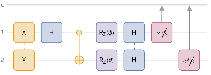 |
Generate the multivariate distribution of measurement results based on the assumption that the angles are real:
| In[3]:= |
| Out[4]= |
Calculate the quantum correlation P00-P10-P01+P11
| In[5]:= |
| Out[5]= |
Create the quantum phase estimation circuit for a phase operator:
| In[6]:= | ![qc = InterpretationBox[FrameBox[TagBox[TooltipBox[PaneBox[GridBox[List[List[GraphicsBox[List[Thickness[0.0025`], List[FaceForm[List[RGBColor[0.9607843137254902`, 0.5058823529411764`, 0.19607843137254902`], Opacity[1.`]]], FilledCurveBox[List[List[List[0, 2, 0], List[0, 1, 0], List[0, 1, 0], List[0, 1, 0], List[0, 1, 0]], List[List[0, 2, 0], List[0, 1, 0], List[0, 1, 0], List[0, 1, 0], List[0, 1, 0]], List[List[0, 2, 0], List[0, 1, 0], List[0, 1, 0], List[0, 1, 0], List[0, 1, 0], List[0, 1, 0]], List[List[0, 2, 0], List[1, 3, 3], List[0, 1, 0], List[1, 3, 3], List[0, 1, 0], List[1, 3, 3], List[0, 1, 0], List[1, 3, 3], List[1, 3, 3], List[0, 1, 0], List[1, 3, 3], List[0, 1, 0], List[1, 3, 3]]], List[List[List[205.`, 22.863691329956055`], List[205.`, 212.31669425964355`], List[246.01799774169922`, 235.99870109558105`], List[369.0710144042969`, 307.0436840057373`], List[369.0710144042969`, 117.59068870544434`], List[205.`, 22.863691329956055`]], List[List[30.928985595703125`, 307.0436840057373`], List[153.98200225830078`, 235.99870109558105`], List[195.`, 212.31669425964355`], List[195.`, 22.863691329956055`], List[30.928985595703125`, 117.59068870544434`], List[30.928985595703125`, 307.0436840057373`]], List[List[200.`, 410.42970085144043`], List[364.0710144042969`, 315.7036876678467`], List[241.01799774169922`, 244.65868949890137`], List[200.`, 220.97669792175293`], List[158.98200225830078`, 244.65868949890137`], List[35.928985595703125`, 315.7036876678467`], List[200.`, 410.42970085144043`]], List[List[376.5710144042969`, 320.03370475769043`], List[202.5`, 420.53370475769043`], List[200.95300006866455`, 421.42667961120605`], List[199.04699993133545`, 421.42667961120605`], List[197.5`, 420.53370475769043`], List[23.428985595703125`, 320.03370475769043`], List[21.882003784179688`, 319.1406993865967`], List[20.928985595703125`, 317.4896984100342`], List[20.928985595703125`, 315.7036876678467`], List[20.928985595703125`, 114.70369529724121`], List[20.928985595703125`, 112.91769218444824`], List[21.882003784179688`, 111.26669120788574`], List[23.428985595703125`, 110.37369346618652`], List[197.5`, 9.87369155883789`], List[198.27300024032593`, 9.426692008972168`], List[199.13700008392334`, 9.203690528869629`], List[200.`, 9.203690528869629`], List[200.86299991607666`, 9.203690528869629`], List[201.72699999809265`, 9.426692008972168`], List[202.5`, 9.87369155883789`], List[376.5710144042969`, 110.37369346618652`], List[378.1179962158203`, 111.26669120788574`], List[379.0710144042969`, 112.91769218444824`], List[379.0710144042969`, 114.70369529724121`], List[379.0710144042969`, 315.7036876678467`], List[379.0710144042969`, 317.4896984100342`], List[378.1179962158203`, 319.1406993865967`], List[376.5710144042969`, 320.03370475769043`]]]]], List[FaceForm[List[RGBColor[0.5529411764705883`, 0.6745098039215687`, 0.8117647058823529`], Opacity[1.`]]], FilledCurveBox[List[List[List[0, 2, 0], List[0, 1, 0], List[0, 1, 0], List[0, 1, 0]]], List[List[List[44.92900085449219`, 282.59088134765625`], List[181.00001525878906`, 204.0298843383789`], List[181.00001525878906`, 46.90887451171875`], List[44.92900085449219`, 125.46986389160156`], List[44.92900085449219`, 282.59088134765625`]]]]], List[FaceForm[List[RGBColor[0.6627450980392157`, 0.803921568627451`, 0.5686274509803921`], Opacity[1.`]]], FilledCurveBox[List[List[List[0, 2, 0], List[0, 1, 0], List[0, 1, 0], List[0, 1, 0]]], List[List[List[355.0710144042969`, 282.59088134765625`], List[355.0710144042969`, 125.46986389160156`], List[219.`, 46.90887451171875`], List[219.`, 204.0298843383789`], List[355.0710144042969`, 282.59088134765625`]]]]], List[FaceForm[List[RGBColor[0.6901960784313725`, 0.5882352941176471`, 0.8117647058823529`], Opacity[1.`]]], FilledCurveBox[List[List[List[0, 2, 0], List[0, 1, 0], List[0, 1, 0], List[0, 1, 0]]], List[List[List[200.`, 394.0606994628906`], List[336.0710144042969`, 315.4997024536133`], List[200.`, 236.93968200683594`], List[63.928985595703125`, 315.4997024536133`], List[200.`, 394.0606994628906`]]]]]], List[Rule[BaselinePosition, Scaled[0.15`]], Rule[ImageSize, 10], Rule[ImageSize, 15]]], StyleBox[RowBox[List["QuantumCircuitOperator", " "]], Rule[ShowAutoStyles, False], Rule[ShowStringCharacters, False], Rule[FontSize, Times[0.9`, Inherited]], Rule[FontColor, GrayLevel[0.1`]]]]], Rule[GridBoxSpacings, List[Rule["Columns", List[List[0.25`]]]]]], Rule[Alignment, List[Left, Baseline]], Rule[BaselinePosition, Baseline], Rule[FrameMargins, List[List[3, 0], List[0, 0]]], Rule[BaseStyle, List[Rule[LineSpacing, List[0, 0]], Rule[LineBreakWithin, False]]]], RowBox[List["PacletSymbol", "[", RowBox[List["\"Wolfram/QuantumFramework\"", ",", "\"Wolfram`QuantumFramework`QuantumCircuitOperator\""]], "]"]], Rule[TooltipStyle, List[Rule[ShowAutoStyles, True], Rule[ShowStringCharacters, True]]]], Function[Annotation[Slot[1], Style[Defer[PacletSymbol["Wolfram/QuantumFramework", "Wolfram`QuantumFramework`QuantumCircuitOperator"]], Rule[ShowStringCharacters, True]], "Tooltip"]]], Rule[Background, RGBColor[0.968`, 0.976`, 0.984`]], Rule[BaselinePosition, Baseline], Rule[DefaultBaseStyle, List[]], Rule[FrameMargins, List[List[0, 0], List[1, 1]]], Rule[FrameStyle, RGBColor[0.831`, 0.847`, 0.85`]], Rule[RoundingRadius, 4]], PacletSymbol["Wolfram/QuantumFramework", "Wolfram`QuantumFramework`QuantumCircuitOperator"], Rule[Selectable, False], Rule[SelectWithContents, True], Rule[BoxID, "PacletSymbolBox"]][{"PhaseEstimation", InterpretationBox[FrameBox[TagBox[TooltipBox[PaneBox[GridBox[List[List[GraphicsBox[List[Thickness[0.0025`], List[FaceForm[List[RGBColor[0.9607843137254902`, 0.5058823529411764`, 0.19607843137254902`], Opacity[1.`]]], FilledCurveBox[List[List[List[0, 2, 0], List[0, 1, 0], List[0, 1, 0], List[0, 1, 0], List[0, 1, 0]], List[List[0, 2, 0], List[0, 1, 0], List[0, 1, 0], List[0, 1, 0], List[0, 1, 0]], List[List[0, 2, 0], List[0, 1, 0], List[0, 1, 0], List[0, 1, 0], List[0, 1, 0], List[0, 1, 0]], List[List[0, 2, 0], List[1, 3, 3], List[0, 1, 0], List[1, 3, 3], List[0, 1, 0], List[1, 3, 3], List[0, 1, 0], List[1, 3, 3], List[1, 3, 3], List[0, 1, 0], List[1, 3, 3], List[0, 1, 0], List[1, 3, 3]]], List[List[List[205.`, 22.863691329956055`], List[205.`, 212.31669425964355`], List[246.01799774169922`, 235.99870109558105`], List[369.0710144042969`, 307.0436840057373`], List[369.0710144042969`, 117.59068870544434`], List[205.`, 22.863691329956055`]], List[List[30.928985595703125`, 307.0436840057373`], List[153.98200225830078`, 235.99870109558105`], List[195.`, 212.31669425964355`], List[195.`, 22.863691329956055`], List[30.928985595703125`, 117.59068870544434`], List[30.928985595703125`, 307.0436840057373`]], List[List[200.`, 410.42970085144043`], List[364.0710144042969`, 315.7036876678467`], List[241.01799774169922`, 244.65868949890137`], List[200.`, 220.97669792175293`], List[158.98200225830078`, 244.65868949890137`], List[35.928985595703125`, 315.7036876678467`], List[200.`, 410.42970085144043`]], List[List[376.5710144042969`, 320.03370475769043`], List[202.5`, 420.53370475769043`], List[200.95300006866455`, 421.42667961120605`], List[199.04699993133545`, 421.42667961120605`], List[197.5`, 420.53370475769043`], List[23.428985595703125`, 320.03370475769043`], List[21.882003784179688`, 319.1406993865967`], List[20.928985595703125`, 317.4896984100342`], List[20.928985595703125`, 315.7036876678467`], List[20.928985595703125`, 114.70369529724121`], List[20.928985595703125`, 112.91769218444824`], List[21.882003784179688`, 111.26669120788574`], List[23.428985595703125`, 110.37369346618652`], List[197.5`, 9.87369155883789`], List[198.27300024032593`, 9.426692008972168`], List[199.13700008392334`, 9.203690528869629`], List[200.`, 9.203690528869629`], List[200.86299991607666`, 9.203690528869629`], List[201.72699999809265`, 9.426692008972168`], List[202.5`, 9.87369155883789`], List[376.5710144042969`, 110.37369346618652`], List[378.1179962158203`, 111.26669120788574`], List[379.0710144042969`, 112.91769218444824`], List[379.0710144042969`, 114.70369529724121`], List[379.0710144042969`, 315.7036876678467`], List[379.0710144042969`, 317.4896984100342`], List[378.1179962158203`, 319.1406993865967`], List[376.5710144042969`, 320.03370475769043`]]]]], List[FaceForm[List[RGBColor[0.5529411764705883`, 0.6745098039215687`, 0.8117647058823529`], Opacity[1.`]]], FilledCurveBox[List[List[List[0, 2, 0], List[0, 1, 0], List[0, 1, 0], List[0, 1, 0]]], List[List[List[44.92900085449219`, 282.59088134765625`], List[181.00001525878906`, 204.0298843383789`], List[181.00001525878906`, 46.90887451171875`], List[44.92900085449219`, 125.46986389160156`], List[44.92900085449219`, 282.59088134765625`]]]]], List[FaceForm[List[RGBColor[0.6627450980392157`, 0.803921568627451`, 0.5686274509803921`], Opacity[1.`]]], FilledCurveBox[List[List[List[0, 2, 0], List[0, 1, 0], List[0, 1, 0], List[0, 1, 0]]], List[List[List[355.0710144042969`, 282.59088134765625`], List[355.0710144042969`, 125.46986389160156`], List[219.`, 46.90887451171875`], List[219.`, 204.0298843383789`], List[355.0710144042969`, 282.59088134765625`]]]]], List[FaceForm[List[RGBColor[0.6901960784313725`, 0.5882352941176471`, 0.8117647058823529`], Opacity[1.`]]], FilledCurveBox[List[List[List[0, 2, 0], List[0, 1, 0], List[0, 1, 0], List[0, 1, 0]]], List[List[List[200.`, 394.0606994628906`], List[336.0710144042969`, 315.4997024536133`], List[200.`, 236.93968200683594`], List[63.928985595703125`, 315.4997024536133`], List[200.`, 394.0606994628906`]]]]]], List[Rule[BaselinePosition, Scaled[0.15`]], Rule[ImageSize, 10], Rule[ImageSize, 15]]], StyleBox[RowBox[List["QuantumOperator", " "]], Rule[ShowAutoStyles, False], Rule[ShowStringCharacters, False], Rule[FontSize, Times[0.9`, Inherited]], Rule[FontColor, GrayLevel[0.1`]]]]], Rule[GridBoxSpacings, List[Rule["Columns", List[List[0.25`]]]]]], Rule[Alignment, List[Left, Baseline]], Rule[BaselinePosition, Baseline], Rule[FrameMargins, List[List[3, 0], List[0, 0]]], Rule[BaseStyle, List[Rule[LineSpacing, List[0, 0]], Rule[LineBreakWithin, False]]]], RowBox[List["PacletSymbol", "[", RowBox[List["\"Wolfram/QuantumFramework\"", ",", "\"Wolfram`QuantumFramework`QuantumOperator\""]], "]"]], Rule[TooltipStyle, List[Rule[ShowAutoStyles, True], Rule[ShowStringCharacters, True]]]], Function[Annotation[Slot[1], Style[Defer[PacletSymbol["Wolfram/QuantumFramework", "Wolfram`QuantumFramework`QuantumOperator"]], Rule[ShowStringCharacters, True]], "Tooltip"]]], Rule[Background, RGBColor[0.968`, 0.976`, 0.984`]], Rule[BaselinePosition, Baseline], Rule[DefaultBaseStyle, List[]], Rule[FrameMargins, List[List[0, 0], List[1, 1]]], Rule[FrameStyle, RGBColor[0.831`, 0.847`, 0.85`]], Rule[RoundingRadius, 4]], PacletSymbol["Wolfram/QuantumFramework", "Wolfram`QuantumFramework`QuantumOperator"], Rule[Selectable, False], Rule[SelectWithContents, True], Rule[BoxID, "PacletSymbolBox"]][{"Phase", 2 \[Pi]/5}], 4}];
qc["Diagram"]](https://www.wolframcloud.com/obj/resourcesystem/images/b7a/b7acdc31-f5bd-43d2-a50f-580e75215231/47243785c188fe54.png) |
| Out[7]= | 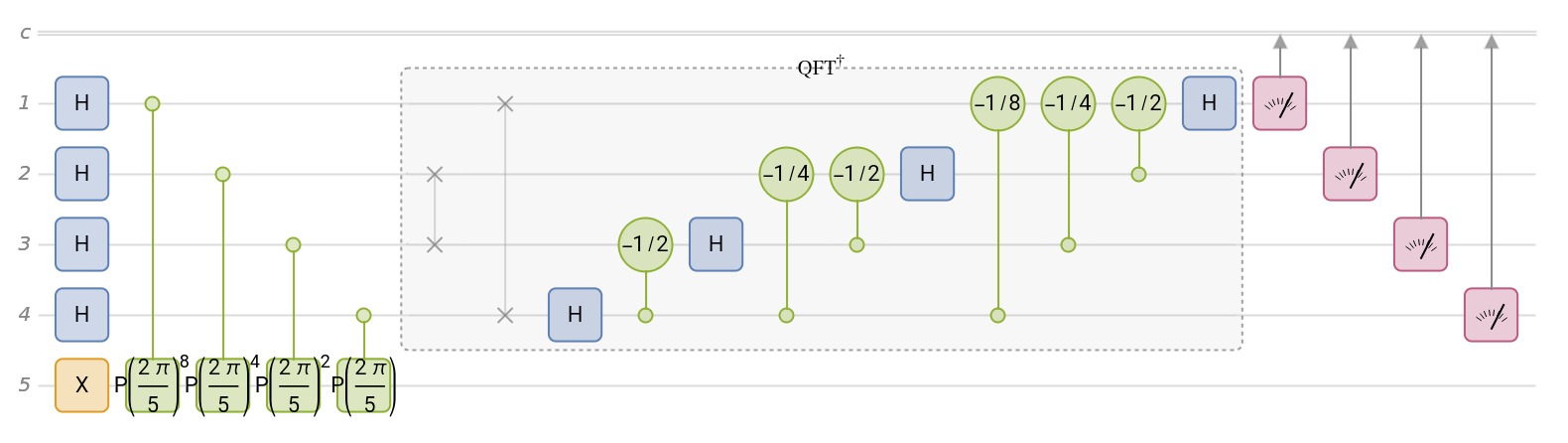 |
| In[8]:= |
| Out[8]= |
| In[9]:= |
| Out[9]= |  |
Set time and other variables of the Hamiltonian (Rabi drive and detuning):
| In[10]:= | ![\[CapitalOmega] = 15. Sin[t]^2;
\[CapitalDelta] = 10. Sin[t - 1];
Plot[{\[CapitalOmega], \[CapitalDelta]}, {t, 0, 3}, PlotLegends -> {"\[CapitalOmega]", "\[CapitalDelta]"}, AspectRatio -> 1/2]](https://www.wolframcloud.com/obj/resourcesystem/images/b7a/b7acdc31-f5bd-43d2-a50f-580e75215231/17661264edfe66c9.png) |
| Out[12]= | 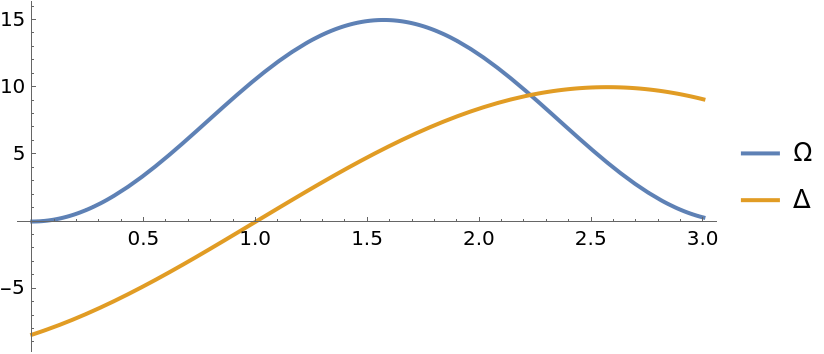 |
Create a 10-qubit Hamiltonian operator as ![]()
| In[13]:= |
Evolve quantum state:
| In[14]:= |
Plot the probability of observing the register state:
| In[15]:= | ![Plot[Evaluate@Normal@\[Psi]["ProbabilitiesList"], {t, 0, 3.}, PlotLabel -> "Population vs time", PlotLegends -> {Ket[{0}], Ket[{1}]},
AspectRatio -> 1/2]](https://www.wolframcloud.com/obj/resourcesystem/images/b7a/b7acdc31-f5bd-43d2-a50f-580e75215231/57f8b6b3980892c0.png) |
| Out[15]= | 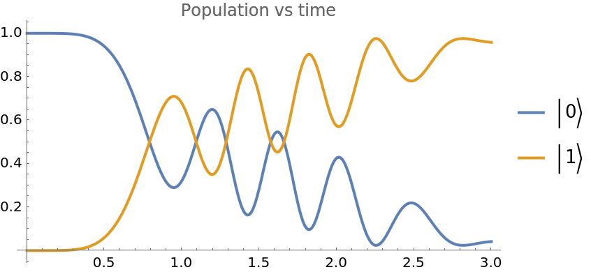 |
Plot the Bloch vector evolution:
| In[16]:= | ![Show[InterpretationBox[FrameBox[TagBox[TooltipBox[PaneBox[GridBox[List[List[GraphicsBox[List[Thickness[0.0025`], List[FaceForm[List[RGBColor[0.9607843137254902`, 0.5058823529411764`, 0.19607843137254902`], Opacity[1.`]]], FilledCurveBox[List[List[List[0, 2, 0], List[0, 1, 0], List[0, 1, 0], List[0, 1, 0], List[0, 1, 0]], List[List[0, 2, 0], List[0, 1, 0], List[0, 1, 0], List[0, 1, 0], List[0, 1, 0]], List[List[0, 2, 0], List[0, 1, 0], List[0, 1, 0], List[0, 1, 0], List[0, 1, 0], List[0, 1, 0]], List[List[0, 2, 0], List[1, 3, 3], List[0, 1, 0], List[1, 3, 3], List[0, 1, 0], List[1, 3, 3], List[0, 1, 0], List[1, 3, 3], List[1, 3, 3], List[0, 1, 0], List[1, 3, 3], List[0, 1, 0], List[1, 3, 3]]], List[List[List[205.`, 22.863691329956055`], List[205.`, 212.31669425964355`], List[246.01799774169922`, 235.99870109558105`], List[369.0710144042969`, 307.0436840057373`], List[369.0710144042969`, 117.59068870544434`], List[205.`, 22.863691329956055`]], List[List[30.928985595703125`, 307.0436840057373`], List[153.98200225830078`, 235.99870109558105`], List[195.`, 212.31669425964355`], List[195.`, 22.863691329956055`], List[30.928985595703125`, 117.59068870544434`], List[30.928985595703125`, 307.0436840057373`]], List[List[200.`, 410.42970085144043`], List[364.0710144042969`, 315.7036876678467`], List[241.01799774169922`, 244.65868949890137`], List[200.`, 220.97669792175293`], List[158.98200225830078`, 244.65868949890137`], List[35.928985595703125`, 315.7036876678467`], List[200.`, 410.42970085144043`]], List[List[376.5710144042969`, 320.03370475769043`], List[202.5`, 420.53370475769043`], List[200.95300006866455`, 421.42667961120605`], List[199.04699993133545`, 421.42667961120605`], List[197.5`, 420.53370475769043`], List[23.428985595703125`, 320.03370475769043`], List[21.882003784179688`, 319.1406993865967`], List[20.928985595703125`, 317.4896984100342`], List[20.928985595703125`, 315.7036876678467`], List[20.928985595703125`, 114.70369529724121`], List[20.928985595703125`, 112.91769218444824`], List[21.882003784179688`, 111.26669120788574`], List[23.428985595703125`, 110.37369346618652`], List[197.5`, 9.87369155883789`], List[198.27300024032593`, 9.426692008972168`], List[199.13700008392334`, 9.203690528869629`], List[200.`, 9.203690528869629`], List[200.86299991607666`, 9.203690528869629`], List[201.72699999809265`, 9.426692008972168`], List[202.5`, 9.87369155883789`], List[376.5710144042969`, 110.37369346618652`], List[378.1179962158203`, 111.26669120788574`], List[379.0710144042969`, 112.91769218444824`], List[379.0710144042969`, 114.70369529724121`], List[379.0710144042969`, 315.7036876678467`], List[379.0710144042969`, 317.4896984100342`], List[378.1179962158203`, 319.1406993865967`], List[376.5710144042969`, 320.03370475769043`]]]]], List[FaceForm[List[RGBColor[0.5529411764705883`, 0.6745098039215687`, 0.8117647058823529`], Opacity[1.`]]], FilledCurveBox[List[List[List[0, 2, 0], List[0, 1, 0], List[0, 1, 0], List[0, 1, 0]]], List[List[List[44.92900085449219`, 282.59088134765625`], List[181.00001525878906`, 204.0298843383789`], List[181.00001525878906`, 46.90887451171875`], List[44.92900085449219`, 125.46986389160156`], List[44.92900085449219`, 282.59088134765625`]]]]], List[FaceForm[List[RGBColor[0.6627450980392157`, 0.803921568627451`, 0.5686274509803921`], Opacity[1.`]]], FilledCurveBox[List[List[List[0, 2, 0], List[0, 1, 0], List[0, 1, 0], List[0, 1, 0]]], List[List[List[355.0710144042969`, 282.59088134765625`], List[355.0710144042969`, 125.46986389160156`], List[219.`, 46.90887451171875`], List[219.`, 204.0298843383789`], List[355.0710144042969`, 282.59088134765625`]]]]], List[FaceForm[List[RGBColor[0.6901960784313725`, 0.5882352941176471`, 0.8117647058823529`], Opacity[1.`]]], FilledCurveBox[List[List[List[0, 2, 0], List[0, 1, 0], List[0, 1, 0], List[0, 1, 0]]], List[List[List[200.`, 394.0606994628906`], List[336.0710144042969`, 315.4997024536133`], List[200.`, 236.93968200683594`], List[63.928985595703125`, 315.4997024536133`], List[200.`, 394.0606994628906`]]]]]], List[Rule[BaselinePosition, Scaled[0.15`]], Rule[ImageSize, 10], Rule[ImageSize, 15]]], StyleBox[RowBox[List["QuantumState", " "]], Rule[ShowAutoStyles, False], Rule[ShowStringCharacters, False], Rule[FontSize, Times[0.9`, Inherited]], Rule[FontColor, GrayLevel[0.1`]]]]], Rule[GridBoxSpacings, List[Rule["Columns", List[List[0.25`]]]]]], Rule[Alignment, List[Left, Baseline]], Rule[BaselinePosition, Baseline], Rule[FrameMargins, List[List[3, 0], List[0, 0]]], Rule[BaseStyle, List[Rule[LineSpacing, List[0, 0]], Rule[LineBreakWithin, False]]]], RowBox[List["PacletSymbol", "[", RowBox[List["\"Wolfram/QuantumFramework\"", ",", "\"Wolfram`QuantumFramework`QuantumState\""]], "]"]], Rule[TooltipStyle, List[Rule[ShowAutoStyles, True], Rule[ShowStringCharacters, True]]]], Function[Annotation[Slot[1], Style[Defer[PacletSymbol["Wolfram/QuantumFramework", "Wolfram`QuantumFramework`QuantumState"]], Rule[ShowStringCharacters, True]], "Tooltip"]]], Rule[Background, RGBColor[0.968`, 0.976`, 0.984`]], Rule[BaselinePosition, Baseline], Rule[DefaultBaseStyle, List[]], Rule[FrameMargins, List[List[0, 0], List[1, 1]]], Rule[FrameStyle, RGBColor[0.831`, 0.847`, 0.85`]], Rule[RoundingRadius, 4]], PacletSymbol["Wolfram/QuantumFramework", "Wolfram`QuantumFramework`QuantumState"], Rule[Selectable, False], Rule[SelectWithContents, True], Rule[BoxID, "PacletSymbolBox"]]["UniformMixture"][
"BlochPlot"], ParametricPlot3D[\[Psi]["BlochVector"], {t, 0, 3}]]](https://www.wolframcloud.com/obj/resourcesystem/images/b7a/b7acdc31-f5bd-43d2-a50f-580e75215231/37334e661cefd4cd.png) |
| Out[16]= | 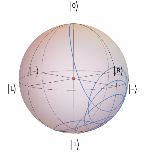 |
Wolfram Language Version 13.1