Wolfram Language Paclet Repository

Community-contributed installable additions to the Wolfram Language

Primary Navigation

    • Cloud & Deployment
    • Core Language & Structure
    • Data Manipulation & Analysis
    • Engineering Data & Computation
    • External Interfaces & Connections
    • Financial Data & Computation
    • Geographic Data & Computation
    • Geometry
    • Graphs & Networks
    • Higher Mathematical Computation
    • Images
    • Knowledge Representation & Natural Language
    • Machine Learning
    • Notebook Documents & Presentation
    • Scientific and Medical Data & Computation
    • Social, Cultural & Linguistic Data
    • Strings & Text
    • Symbolic & Numeric Computation
    • System Operation & Setup
    • Time-Related Computation
    • User Interface Construction
    • Visualization & Graphics
    • Random Paclet
    • Alphabetical List
  • Using Paclets
    • Get Started
    • Download Definition Notebook
  • Learn More about Wolfram Language

QuantumPlaybook

Guides

  • QuantumPlaybook

Tech Notes

  • Addition of Numbers
  • Baker-Hausdorff Lemma
  • Chiral Fermion Random Circuit
  • Clifford Operators: How to Test
  • Commutation Relations for Qubits
  • Entanglement Distillation
  • Generalized Pauli Operators: Implementation
  • Hatano-Nelson-Kitaev Model: Monte Carlo Simulation
  • Hatano-Nelson Model: Monte Carlo Simulation
  • Kitaev Chain
  • Kitaev Random Circuit
  • Λ-Matter in a Cavity
  • Measurement of Total Pauli Z
  • Non-Unitary Dynamics of Quantum States
  • Partial Trace: Physical Meaning
  • Quantum Dot Systems
  • A Quantum Playbook
  • Magnetic Exchange Coupling
  • Solovay-Kitaev Algorithm
  • Spin Code
  • Symmetry Effects On Quantum Master Equations
  • Transmon: Quantum Phase Model
  • Transposition as a Supermap
  • Variational Quantum Classifier: Iris
  • Variational Quantum Classifier: Parity
  • Variational Quantum Eigensolver: Transverse-Field Ising Model

Symbols

  • BlochEnergy
  • BlochFunction
  • QuantumPlaybookCheckUpdate
  • QuantumPlaybookEdition
  • QuantumPlaybookUpdate
  • TransmonEnergy
  • TransmonExponent
  • TransmonFunction
  • TransmonHamiltonian
Entanglement Distillation
To Generate Partially Entangled Pairs
Transformation
Measurement of Total Pauli Z
Overall
See also Section 7.3 of the
Quantum Workbook (Springer, 2022)
.
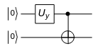
Here, we start with a number of partially entangled pairs and “distills” a smaller number of maximally entangled pairs. This is illustrated in the quantum circuit model.
VonNeumannEntropy
VonNeumann entropy of a mixed state
PartialTrace
Partial trace over some subsystems
Dyad
Dyadic product of two vectors
Functions used in this document.
Make sure that Q3 is loaded.
In[236]:=
Needs["QuantumMob`Q3`"]
We have two parties Alice (A) and Bob (B). Teddy (T) is an ancillary register to perform a measurement of the total Pauli Z.
In[237]:=
Let[Qubit,A,B,T]
We will start with n partially entangled pairs.
In[238]:=
$n=4;​​kk=Range[$n];​​AA=A[kk,$];​​BB=B[kk,$];
You need fewer qubits for T, just enough to store a number up to maximum n.
In[242]:=
ln=Ceiling@Log[2,$n+1];​​TT=T[Range@ln,$];
To Generate Partially Entangled Pairs

A Single Pair

Let us first examine a single pair of partially entangled qubits.
First, construct a superposition of the two computational basis states with different amplitudes.
In[244]:=
Let[Real,ϕ]​​qc=QuantumCircuit[​​Ket[A@{1}],​​Rotation[ϕ,A[1,2]]]
Out[245]=
Parameter ϕ tunes the two amplitudes,
c
0
=cos(ϕ/2)
and
c
1
=sin(ϕ/2)
, in the superposition.
In[246]:=
Elaborate[qc]//ExpandAll
Out[246]=
Cos
ϕ
2

0
A
1
+
1
A
1
Sin
ϕ
2

Then, by applying the CNOT gate, you can create a partially entangled pair.
In[247]:=
qc=QuantumCircuit[​​Ket[{A[1],B[1]}],​​Rotation[ϕ,A[1,2]],​​CNOT[A[1],B[1]]]
Out[247]=
Eventually, we see that the parameter ϕ tunes the extent of entanglement (with
ϕ=π/2
corresponds to the maximal entanglement).
In[248]:=
out=Elaborate[qc]
Out[248]=
Cos
ϕ
2

0
A
1
0
B
1
+
1
A
1
1
B
1
Sin
ϕ
2

Examine the reduced density matrix for the first qubit to check that the above state is partial entangled.
In[249]:=
rho=PartialTrace[out,B[1]]//ExpToTrig//Simplify;​​Matrix[rho]//ExpToTrig//SimplifyThrough//MatrixForm
Out[250]//MatrixForm=
2
Cos
ϕ
2

0
0
2
Sin
ϕ
2


Multiple Pairs

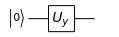
Now, we consider n partially entangled pairs with each pair in the state described above. Let us take a look at the explicit expression for the n partially entangled pairs. Here,
OTimes
is used just for better readability, and you can replace it with
CircleTimes
(⊗) or
Multiply
to get exactly the same result.
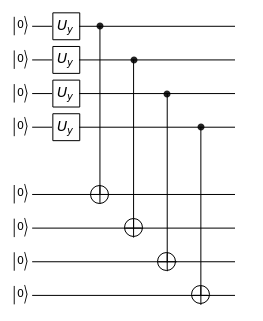
Repeating the above procedure for other pairs, generate as many partially entangled pairs as you like. In this particular example, we prepare four pairs.
In[251]:=
qc0=QuantumCircuit[​​Ket[AA],Ket[BB],​​Rotation[ϕ,A[kk,2]],​​Sequence@@ReleaseHold@Thread@Hold[CNOT][AA,BB],​​"Invisible"A[$n+1/2]​​]
Out[251]=
Expanding it, one gets various terms, each with identical parts on Alice’s and Bob’s side.
In[252]:=
out=Elaborate[qc0];​​ProductForm[out,{AA,BB}]
Out[253]=
4
Cos
ϕ
2

|0000〉⊗|0000〉+
3
Cos
ϕ
2

|0001〉⊗|0001〉Sin
ϕ
2
+|1111〉⊗|1111〉
4
Sin
ϕ
2

+
1
2
2
Cos
ϕ
2

|0100〉⊗|0100〉Sin[ϕ]+
1
2
2
Cos
ϕ
2

|1000〉⊗|1000〉Sin[ϕ]+
1
2
|0111〉⊗|0111〉
2
Sin
ϕ
2

Sin[ϕ]+
1
2
|1011〉⊗|1011〉
2
Sin
ϕ
2

Sin[ϕ]+
1
2
|1101〉⊗|1101〉
2
Sin
ϕ
2

Sin[ϕ]+
1
2
|1110〉⊗|1110〉
2
Sin
ϕ
2

Sin[ϕ]+
1
4
Cot
ϕ
2
|0010〉⊗|0010〉
2
Sin[ϕ]
+
1
4
|0011〉⊗|0011〉
2
Sin[ϕ]
+
1
4
|0101〉⊗|0101〉
2
Sin[ϕ]
+
1
4
|0110〉⊗|0110〉
2
Sin[ϕ]
+
1
4
|1001〉⊗|1001〉
2
Sin[ϕ]
+
1
4
|1010〉⊗|1010〉
2
Sin[ϕ]
+
1
4
|1100〉⊗|1100〉
2
Sin[ϕ]
If Alice (or Bob) measures the total
Z
, i.e.,
Z=
Z
1
+
Z
2
+…+
Z
n
on her qubits (see below), then the possible outcomes are
m=0,1,…,n
and the corresponding probabilities are given by the following formula.
In[254]:=
prb[ϕ_,m_]:=With[{p=Sin[ϕ/2]^2},Binomial[$n,m]*(1-p)^($n-m)p^m]
For fixed
ϕ
, the probability distribution looks like the following plot. The highest probability is for
m=n
2
sin
(ϕ/2)
(
m=3
for
ϕ=2π/3
).
In[255]:=
BarChart[​​Table[prb[2Pi/3,m],{m,$n}],​​ChartLabelsRange[$n],​​AxesNone,FrameTrue,​​FrameLabel{"m","Probability"}​​]
Out[255]=
Measurement of Total Pauli Z
How can we actually measure
Z
tot
:=
Z
1
+
Z
2
+…+
Z
n
on Bob's (or, equivalently, Alice's) qubits.
This is a tiny utility function for convenience.
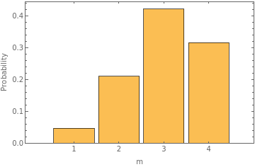
Let us check that the above quantum circuit indeed gives the sum of the bit values of the Bob’s qubits.
Transformation
To get the unitary transformation on Alice's side, we first rearrange the computational basis to get a new basis

Method 1: Using Dyad

These are the computational bases for Alice's and Bob's registers, respectively.
Finally, the unitary transformation is constructed as prescribed above.
By construction, the unitary transformations are just permutation, which is clear from their matrix representations.
Check that they are indeed unitary transformations.

Method 2: Using Permutation

Here, we find the permutation corresponding to the required basis change and use it to construct the unitary matrix.
Construct the operators corresponding to the above matrix.
Examine if the operator properly maps the computational basis states for Alice's qubits.
Also examine if the operator properly maps the computational basis states for Bob's qubits.
Overall
Now, we have all components. Our desired quantum circuit is as follows. The first part generates four partially entangled pairs, the second measures the total Pauli Z on Bob's register, and the last transforms the post-measurement state a fixed pair of qubits from Alice's and Bob's registers.
Here is the output state of the total system. Obviously, the whole register T is separated from the other two registers. So are the last two registers of the respective registers A and B.
Focusing on the first two qubits of registers A and B, we see that there are two maximally entangled pairs.

Remark

then there is no way to turn this state into a product state on a system of qubits.

© 2025 Wolfram. All rights reserved.

  • Legal & Privacy Policy
  • Contact Us
  • WolframAlpha.com
  • WolframCloud.com