Wolfram Language Paclet Repository

Community-contributed installable additions to the Wolfram Language

Primary Navigation

    • Cloud & Deployment
    • Core Language & Structure
    • Data Manipulation & Analysis
    • Engineering Data & Computation
    • External Interfaces & Connections
    • Financial Data & Computation
    • Geographic Data & Computation
    • Geometry
    • Graphs & Networks
    • Higher Mathematical Computation
    • Images
    • Knowledge Representation & Natural Language
    • Machine Learning
    • Notebook Documents & Presentation
    • Scientific and Medical Data & Computation
    • Social, Cultural & Linguistic Data
    • Strings & Text
    • Symbolic & Numeric Computation
    • System Operation & Setup
    • Time-Related Computation
    • User Interface Construction
    • Visualization & Graphics
    • Random Paclet
    • Alphabetical List
  • Using Paclets
    • Get Started
    • Download Definition Notebook
  • Learn More about Wolfram Language

QuantumPlaybook

Guides

  • QuantumPlaybook

Tech Notes

  • Addition of Numbers
  • Baker-Hausdorff Lemma
  • Chiral Fermion Random Circuit
  • Clifford Operators: How to Test
  • Commutation Relations for Qubits
  • Entanglement Distillation
  • Generalized Pauli Operators: Implementation
  • Hatano-Nelson-Kitaev Model: Monte Carlo Simulation
  • Hatano-Nelson Model: Monte Carlo Simulation
  • Kitaev Chain
  • Kitaev Random Circuit
  • Λ-Matter in a Cavity
  • Measurement of Total Pauli Z
  • Non-Unitary Dynamics of Quantum States
  • Partial Trace: Physical Meaning
  • Quantum Dot Systems
  • A Quantum Playbook
  • Magnetic Exchange Coupling
  • Solovay-Kitaev Algorithm
  • Spin Code
  • Symmetry Effects On Quantum Master Equations
  • Transmon: Quantum Phase Model
  • Transposition as a Supermap
  • Variational Quantum Classifier: Iris
  • Variational Quantum Classifier: Parity
  • Variational Quantum Eigensolver: Transverse-Field Ising Model

Symbols

  • BlochEnergy
  • BlochFunction
  • QuantumPlaybookCheckUpdate
  • QuantumPlaybookEdition
  • QuantumPlaybookUpdate
  • TransmonEnergy
  • TransmonExponent
  • TransmonFunction
  • TransmonHamiltonian
Chiral Fermion Random Circuit
The model
Simulation
Setting up model parameters
Analysis
Here, the effects of random measurements on the entanglement in the Su-Schrieffer-Heeger (SSH) model is investigated. A realization of such chiral fermion random circuit is shown in Figure 1.
Figure 1. A typical form of chiral fermion random circuit. Each line indicates a fermion mode, the unitary gate with label
U
denotes the time-evolution of the SSH model, and the measurement symbols depict the measurement of occupation number of the fermion modes.
This demonstration page was motivated by the phenomenon of measurement-induced entanglement transition, a transition between two distinct phases with the entanglement entropy characterized by area- and volume-law scaling. See also Li, Chen, and Fisher (2018), Skinner, Ruhman, and Nahum (2019), Chan et. al. (2019), Sang et al. (2021), and Weinstein, Bao, and Altman (2022).
WickState
Represents a fermionic Gaussian state
WickUnitary
Represents a Gaussian-type unitary operator
WickOperator
Represents a sequence of linear combinations of Majorana operators
RandomWickCircuitSimulate
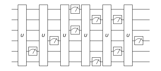
Rancomd quantum circuit consisting of fermionic gates.
WickGreenFunction
Calculates the Green's functions with respect to a Wick state
WickEntanglementEntropy
Calculates the entanglement entropy in a Wick state
WickLogarithmicNegativity
Calculates the logarithmic negativity in a Wick state
Functions for fermionic quantum computation.
The model
In this section, we just examine the model. The material in this section is not directly used in the demonstration from the next section and on. If you are already familiar with the model, you can skip this part.
Make sure to load Q3.
In[44]:=
Needs["QuantumMob`Q3`"]
The bare fermion modes.
In[228]:=
Let[Fermion,c]
Consider a system of n fermion modes.
In[229]:=
$n=6;​​cc=c[Range@$n]​​odd=cc〚1;;;;2〛​​evn=cc〚2;;;;2〛
Out[230]=
{
c
1
,
c
2
,
c
3
,
c
4
,
c
5
,
c
6
}
Out[231]=
{
c
1
,
c
3
,
c
5
}
Out[232]=
{
c
2
,
c
4
,
c
6
}
Construct the many-body Hamiltonian of the SSH model.
In[233]:=
Let[Real,g]
In[234]:=
HH=-g[1]*Hop[{odd,evn}]-g[2]*Hop[{Most@evn,Rest@odd}]​​HH=HH//PlusDagger;
Out[234]=
-
g
2

†
c
2
c
3
+
†
c
4
c
5
-
g
1

†
c
1
c
2
+
†
c
3
c
4
+
†
c
5
c
6

Examine the connectivity between neighboring fermion modes.
In[236]:=
GraphForm[-HH]
Out[236]=
Extract the single-particle (or Bogoliubov-de Gennes) Hamiltonian (cf. many-body Hamiltonian in the above) of the model in the Nambu space.
In[237]:=
matH=CoefficientTensor[HH,Dagger@cc,cc];​​ArrayShort[matH,"Size"8]
Out[238]//MatrixForm=
0
-
g
1
0
0
0
0
-
g
1
0
-
g
2
0
0
0
0
-
g
2
0
-
g
1
0
0
0
0
-
g
1
0
-
g
2
0
0
0
0
-
g
2
0
-
g
1
0
0
0
0
-
g
1
0
Rearrange the rows and columns so that the chiral symmetry of the model becomes clearer; that is, the single-particle Hamiltonian in the block off-diagonal form.
In[239]:=
chi=CoefficientTensor[HH,Dagger@Join[odd,evn],Join[odd,evn]];​​ArrayShort[chi,"Size"8]
Out[240]//MatrixForm=
0
0
0
-
g
1
0
0
0
0
0
-
g
2
-
g
1
0
0
0
0
0
-
g
2
-
g
1
-
g
1
-
g
2
0
0
0
0
0
-
g
1
-
g
2
0
0
0
0
0
-
g
1
0
0
0
Any physical properties of the model is completely determined by the off-diagonal blocks.
In[241]:=
chi=CoefficientTensor[HH,Dagger@odd,evn];​​chi//ArrayShort
Out[242]//MatrixForm=
-
g
1
0
0
-
g
2
-
g
1
0
0
-
g
2
-
g
1
Re-examine the connectivity of the fermionic modes in the model.
In[243]:=
ChiralGraphForm[-chi,VertexLabels{odd,evn}]
Out[243]=
Setting up model parameters
Now, we set up the parameters for the demonstration.
Make sure to load Q3.
In[1]:=
Needs["QuantumMob`Q3`"]
Set the number of fermion modes to consider.
In[2]:=
$n=10;
Directly construct the single-particle Hamiltonian of the SSH model (without using fermion operator algebra as in the above).
In[3]:=
Let[Real,g]
In[4]:=
matH=PadRight[g@{1,2},$n-1,g@{1,2}];​​matH=PlusTopple@DiagonalMatrix[-matH,1];​​ArrayShort[matH,"Size"6]
Out[6]//MatrixForm=
0
-
g
1
0
0
0
0
…
-
g
1
0
-
g
2
0
0
0
…
0
-
g
2
0
-
g
1
0
0
…
0
0
-
g
1
0
-
g
2
0
…
0
0
0
-
g
2
0
-
g
1
…
0
0
0
0
-
g
1
0
…
…
…
…
…
…
…
…
In[7]:=
ham=NambuHermitian[{matH,0}]​​ham//ArrayShort
Out[7]=
NambuHermitian
Target: All
Dimensions: {10,10}

Out[8]=

0
-
g
1
0
0
…
-
g
1
0
-
g
2
0
…
0
-
g
2
0
-
g
1
…
0
0
-
g
1
0
…
…
…
…
…
…
,
0
0
0
0
…
0
0
0
0
…
0
0
0
0
…
0
0
0
0
…
…
…
…
…
…

Convert the above Hamiltonian matrix in the Dirac spinor space to that in the Majorana spinor space.
In[9]:=
ant=WickHermitian[ham]​​ant//ArrayShort
Out[9]=
WickHermitian
Modes: 10
Dimensions: {20,20}

Out[10]//MatrixForm=
0
0
0
-
g
1
…
0
0
g
1
0
…
0
-
g
1
0
0
…
g
1
0
0
0
…
…
…
…
…
…
The time interval for each unitary layer to operate.
The alternating hopping amplitudes.
Construct the single-particle time-evolution matrix.
Construct the corresponding unitary (in fact, real orthogonal) matrix. It has the same information as the above matrix, but operates directly on Wick states.
Prepare an initial state. A half-filling is a common choice.
The probability to perform a measurement on each fermion mode.
The depth of quantum circuit.
Simulation
The simulation involves a lot of random number generators. To get the same result every time you open this document, set the seed of the random number generator.
Examine the structure of the result.
Examine some of the output states as well.
Analysis
Each entry in the data contains the information about one realization of quantum trajectory. Extract the trajectory history in an explicit form, for example, of the first entry.
In this particular case, there are 13 entries; the first entry is just the initial state and the rest are corresponds to the layers; there are 6 layers and each layer contains two sub-layers of unitary evolution and measurements.
Note that the output states are all normalized.

Entanglement Entropy

Take a subsystem containing the first half of the whole modes.
Calculate the entanglement entropy, and take the average over different trajectories.
Plot the entanglement entropy (EE) as a function of time.

Entanglement Entropy: For different sub-system sizes

Now, let us examine the entanglement entropy for subsystems of different sizes. The largest subsystem has a half of the whole modes.
From the Green’s functions, calculate the entanglement entropy for different subsystems, taking the average over all quantum trajectories.
Plot the average entanglement entropy (EE) as a function of time.

Green's Functions

Calculate the Green's functions.

© 2025 Wolfram. All rights reserved.

  • Legal & Privacy Policy
  • Contact Us
  • WolframAlpha.com
  • WolframCloud.com