Basic Examples (2)
Compute the radial distribution function from two points:
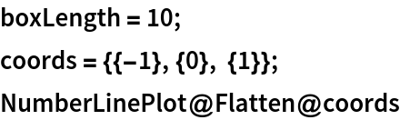
Compute the radial distribution function of a set of coordinates enclosed in a periodic 1D "box" of size (L = 4):
Display the coordinates in number line format along the axis for which the positions differ:
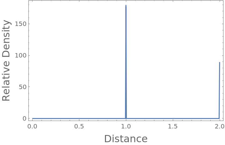
The radial distribution function has nonzero peaks at positions near those of the exact distances apart:
Plot the radial distribution function characteristic of this system:
Options (1)
RadialDistributionFunctionList takes the same options as Compile, and benefits from automated compilation to C:
Applications (2)
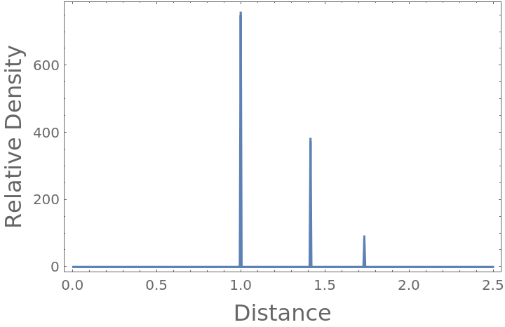
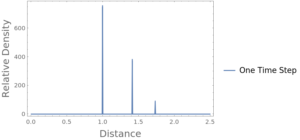
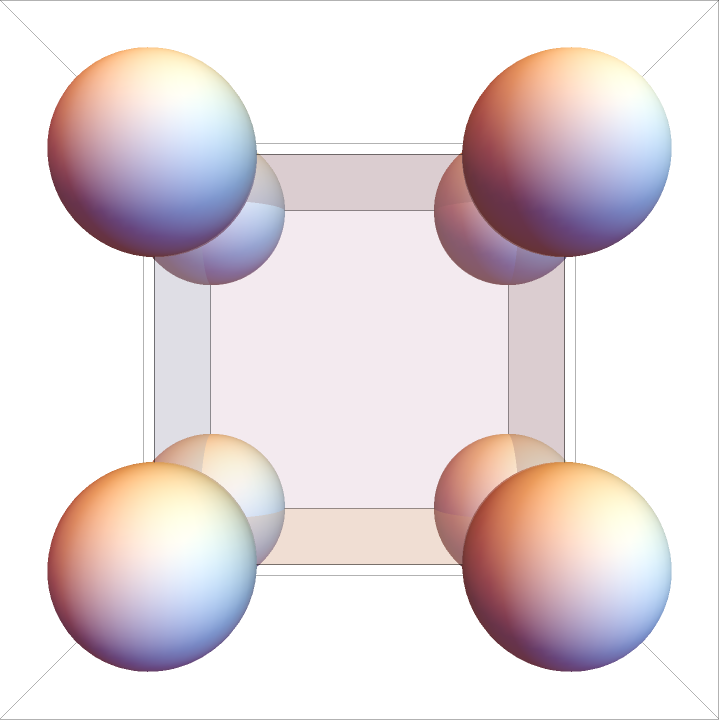
Compute the radial distribution function characteristic of a cube with unit length, enclosed in a sufficiently larger periodic box:
Plot the resulting radial distribution function, where you can see nearest neighbor, polygonal face hypotenuse and internal hypotenuse distances:
Properties and Relations (3)
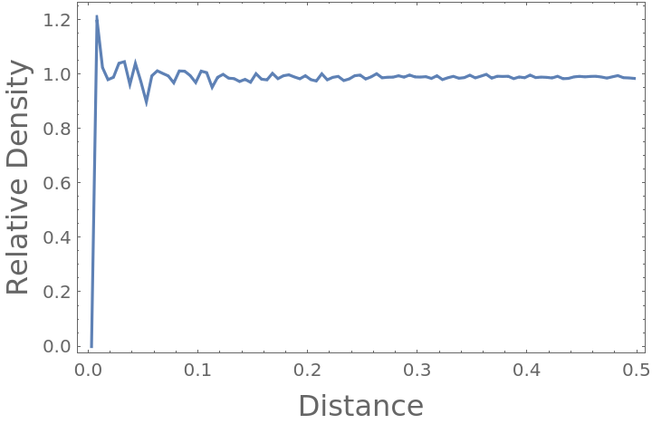
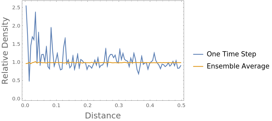
By definition, the radial distribution function of an ideal gas converges to 1 at all distances when provided sufficient data (here, 1000 time steps on 100 positions of 100 particles):
Compute both the radial distribution function of just the first time step, and then that of the ensemble average over all time steps:
As expected, the radial distribution function converges to nearly 1 as sufficient data is introduced:
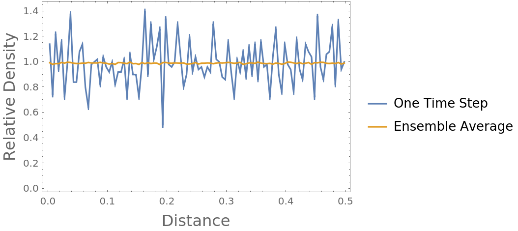
Normalization by the expected number of particles in that vicinity works in 2D cases as well:
The same is true for 1D cases:
Possible Issues (4)
The radial distribution function is accurate out to  and is thus truncated at this point, beyond which it would artificially decay:
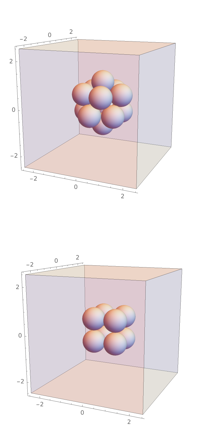
If the box is sufficiently larger than the domain of the particle coordinates, the calculation is as expected (using real particle positions):
The peaks are at the expected unit distance for the touching particles, at the polygonal face hypotenuse distance and the interior hypotenuse:
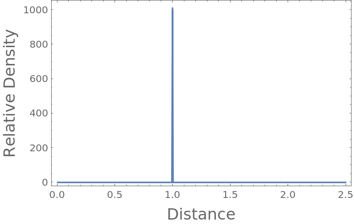
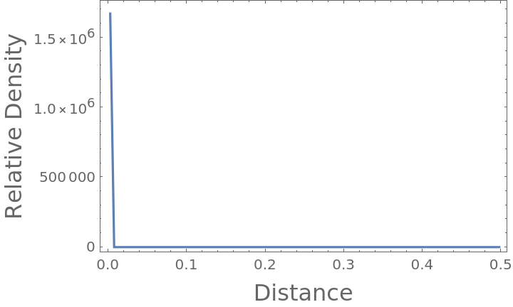
If the box size (L) is too small, the minimum image convention is employed, applying periodicity in each dimension:
In this case, particles are perfectly overlapping and the separation distance between all pairs is rij=0; however, the convention is to put them in the first nonzero bin:
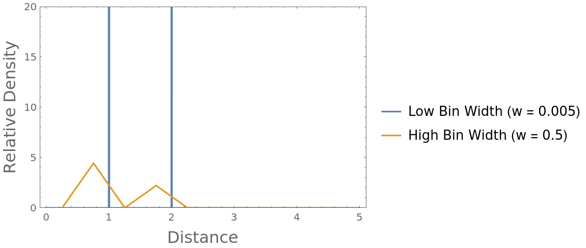
Modifying the concentric shell bin width can affect normalization and positional accuracy, similar to the behavior in Riemann sums with too few discretizing rectangles:
Compare the difference when using two different bin widths:
Neat Examples (3)
Compute the radial distribution function characteristic of an icosahedral distribution of particles and compare it with that of a cube, each with a minimum separation distance of 1:
Plot the resulting radial distribution functions to compare:
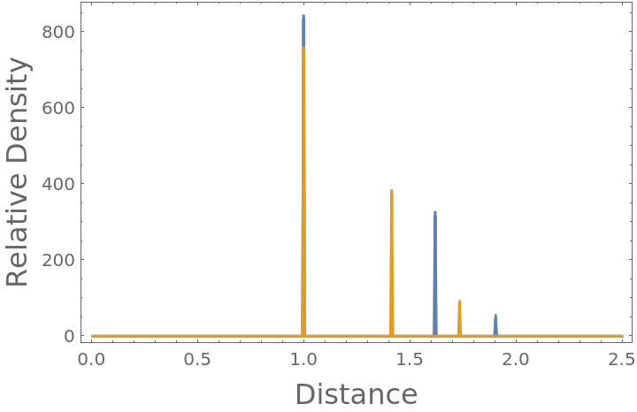
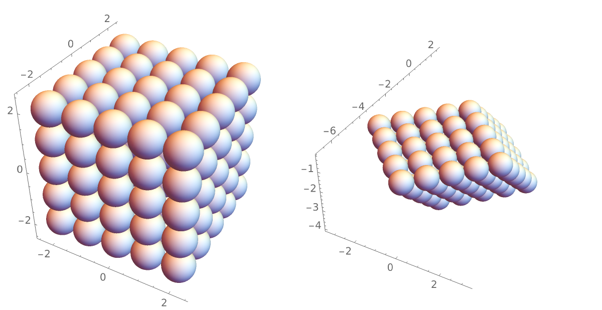
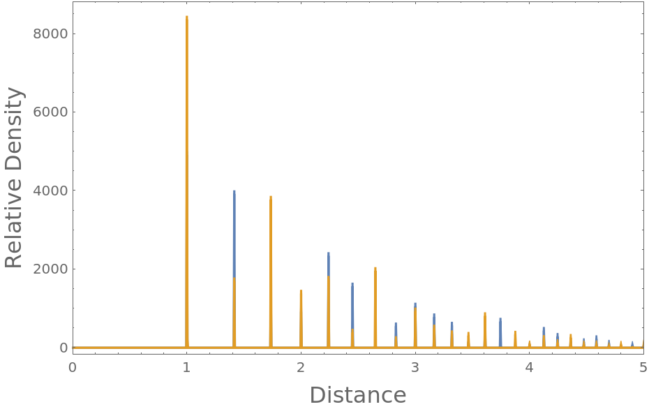
Compare the radial distribution function of both a simple cubic and face-centered cubic (FCC) crystalline lattice (neglecting periodicity, each with nearest neighbors touching at unit lengths):
Compute and plot the radial distribution functions to compare:
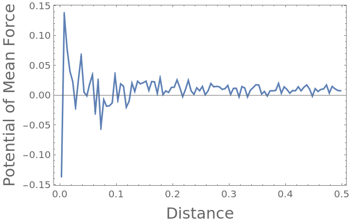
Compute the potential of mean force that has given rise to the interactions, in this example showing that the 3D ideal gas has no potential of interaction:
Compute the corresponding potential of mean force (in units where kBT=1):
It can be seen that despite the noise associated finite data, the potential of mean force is fairly close to zero when averaged over the entire domain:
![boxLength = 5.0;
coords = N@PolyhedronData["Cube", "Vertices"];
rdfData = ResourceFunction["RadialDistributionFunctionList"][coords, boxLength, 0.005];
Graphics3D[{{Opacity[0.25], Cube[boxLength]}, {Sphere[#, 0.5] & /@ coords}}, Sequence[
Boxed -> False, Axes -> True]]](https://www.wolframcloud.com/obj/resourcesystem/images/09e/09e1f52f-c32c-418b-8470-86aa014d597d/1-0-0/193acb7a1751b593.png)

![singleTimestepRDF = ResourceFunction["RadialDistributionFunctionList"][
First@bulkCoordsData, 1.0, 0.005];
ensAvgRDF = Mean[Map[ResourceFunction["RadialDistributionFunctionList"][#, 1.0, 0.005] &, bulkCoordsData]];](https://www.wolframcloud.com/obj/resourcesystem/images/09e/09e1f52f-c32c-418b-8470-86aa014d597d/1-0-0/1d0a511e51279a21.png)
![bulkCoordsData = Table[RandomReal[{0, 1.}, 2], {1000}, {100}];
singleTimestepRDF = ResourceFunction["RadialDistributionFunctionList"][
First@bulkCoordsData, 1.0, 0.005];
ensAvgRDF = Mean[Map[ResourceFunction["RadialDistributionFunctionList"][#, 1.0, 0.005] &, bulkCoordsData]];](https://www.wolframcloud.com/obj/resourcesystem/images/09e/09e1f52f-c32c-418b-8470-86aa014d597d/1-0-0/4792b77616c23931.png)

![bulkCoordsData = Table[{RandomReal[{0, 1.}]}, {1000}, {100}];
singleTimestepRDF = ResourceFunction["RadialDistributionFunctionList"][
First@bulkCoordsData, 1.0, 0.005];
ensAvgRDF = Mean[Map[ResourceFunction["RadialDistributionFunctionList"][#, 1.0, 0.005] &, bulkCoordsData]];](https://www.wolframcloud.com/obj/resourcesystem/images/09e/09e1f52f-c32c-418b-8470-86aa014d597d/1-0-0/1308e01a2201d21b.png)
![boxLength = 5;
coords = {{0, 0, 0}, {1, 0, 0}};
rdfData = ResourceFunction["RadialDistributionFunctionList"][coords, boxLength];
ListLinePlot[rdfData, Sequence[
PlotRange -> All, Frame -> True, FrameLabel -> Map[Style[#, 16]& , {"Distance", "Relative Density"}]]
]](https://www.wolframcloud.com/obj/resourcesystem/images/09e/09e1f52f-c32c-418b-8470-86aa014d597d/1-0-0/3c0ca26fc20902fa.png)
![boxLength = 5;
coords = N@PolyhedronData["Cube", "Vertices"];
rdfData = ResourceFunction["RadialDistributionFunctionList"][coords, boxLength, 0.005];
Graphics3D[{{Opacity[0.25], Cube[boxLength]}, {Sphere[#, 0.5] & /@ coords}}, Sequence[
Boxed -> False, Axes -> True]]](https://www.wolframcloud.com/obj/resourcesystem/images/09e/09e1f52f-c32c-418b-8470-86aa014d597d/1-0-0/66596d900a65283f.png)
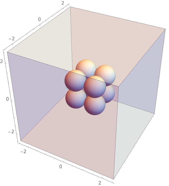
![boxLength = 1;
coords = N@PolyhedronData["Cube", "Vertices"];
rdfData = ResourceFunction["RadialDistributionFunctionList"][coords, boxLength, 0.005];
Graphics3D[{{Opacity[0.25], Cube[boxLength]}, {Sphere[#, 0.25] & /@ coords}}, Sequence[
PlotRange -> All, Frame -> True, FrameLabel -> Map[Style[#, 16]& , {"Distance", "Relative Density"}]]
]](https://www.wolframcloud.com/obj/resourcesystem/images/09e/09e1f52f-c32c-418b-8470-86aa014d597d/1-0-0/544e7f0a0858f3af.png)
![rdfDataLowBinWidth = ResourceFunction["RadialDistributionFunctionList"][coords, boxLength, 0.005];
rdfDataHighBinWidth = ResourceFunction["RadialDistributionFunctionList"][coords, boxLength, 0.5];](https://www.wolframcloud.com/obj/resourcesystem/images/09e/09e1f52f-c32c-418b-8470-86aa014d597d/1-0-0/45f2a948b708cd65.png)
![ListLinePlot[{rdfDataLowBinWidth, rdfDataHighBinWidth}, PlotRange -> {All, {0, 20}}, PlotLegends -> {"Low Bin Width (w = 0.005)", "High Bin Width (w = 0.5)"}, Frame -> True, FrameLabel -> (Style[#1, 16] &) /@ {"Distance", "Relative Density"}]](https://www.wolframcloud.com/obj/resourcesystem/images/09e/09e1f52f-c32c-418b-8470-86aa014d597d/1-0-0/3c340073dd6ef93c.png)
![boxLength = 5;
icosaCoords = N@PolyhedronData["Icosahedron", "Vertices"];
cubeCoords = N@PolyhedronData["Cube", "Vertices"];
rdfData = ResourceFunction["RadialDistributionFunctionList"][#, boxLength, 0.005] & /@ {icosaCoords, cubeCoords};
Row@(Graphics3D[{{Opacity[0.25], Cube[boxLength]}, {Sphere[#, 0.5] & /@ #}}, Boxed -> False, Axes -> True, ViewPoint -> {1.35, -3, 0.8}, ImageSize -> 350] & /@ {icosaCoords, cubeCoords})](https://www.wolframcloud.com/obj/resourcesystem/images/09e/09e1f52f-c32c-418b-8470-86aa014d597d/1-0-0/30d3fc8e150ac240.png)
![cubicCoords = N@Flatten[
Table[{i, j, k}, {i, -2, 2, 1}, {j, -2, 2, 1}, {k, -2, 2, 1}], 2];
\[ScriptCapitalB] = Normal@LatticeData["FaceCenteredCubic", "Basis"];
fccCoords = N@Flatten[
Table[i \[ScriptCapitalB][[1]] + j \[ScriptCapitalB][[2]] + k \[ScriptCapitalB][[3]], {i, 1, 5}, {j, 1, 5}, {k, 1, 5}], 2];
fccCoords = fccCoords/
Min@DeleteCases[Flatten[DistanceMatrix@fccCoords], x_Real /; x == 0.];
Row@(Graphics3D[{{Sphere[#, 0.5] & /@ #}}, Boxed -> False, Axes -> True, ImageSize -> 300] & /@ {cubicCoords, fccCoords})](https://www.wolframcloud.com/obj/resourcesystem/images/09e/09e1f52f-c32c-418b-8470-86aa014d597d/1-0-0/27275ecb36ddbac4.png)
![rdfData = ResourceFunction["RadialDistributionFunctionList"][#, 20, 0.005] & /@ {cubicCoords, fccCoords};
ListLinePlot[rdfData, Sequence[
PlotRange -> {{0, 5}, Automatic}, Frame -> True, FrameLabel -> Map[Style[#, 16]& , {"Distance", "Relative Density"}]]
]](https://www.wolframcloud.com/obj/resourcesystem/images/09e/09e1f52f-c32c-418b-8470-86aa014d597d/1-0-0/2388f467c804cf0b.png)
![bulkCoordsData = Table[RandomReal[{0, 1.}, 3], {1000}, {100}];
ensAvgRDF = Mean[Map[ResourceFunction["RadialDistributionFunctionList"][#, 1.0, 0.005] &, bulkCoordsData]];](https://www.wolframcloud.com/obj/resourcesystem/images/09e/09e1f52f-c32c-418b-8470-86aa014d597d/1-0-0/5365ac7ebacad398.png)