Scope (2)
Other metrics derived from the gyration tensor may be computed:
Metrics may be computed in other dimensions, for example 2D and 4D, respectively:
Properties and Relations (2)
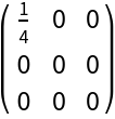
The metrics "NormalizedAsphericity" and "RelativeAnisotropy" have the same limiting behavior in describing spherically symmetric vs. linear distributions:
These metrics do, however, differ in non-limiting cases:
Possible Issues (2)
Available metrics are determined by the dimensions of the input vectors, such that "Acircularity"—a 2D metric—is not computed for 3D:
A given dimension can be omitted to check symmetry in the remaining fewer dimensions:
Non-normalized metrics scale with the size of the distribution:
Normalized equivalents do not and are scaled between 0 and 1:
Neat Examples (8)
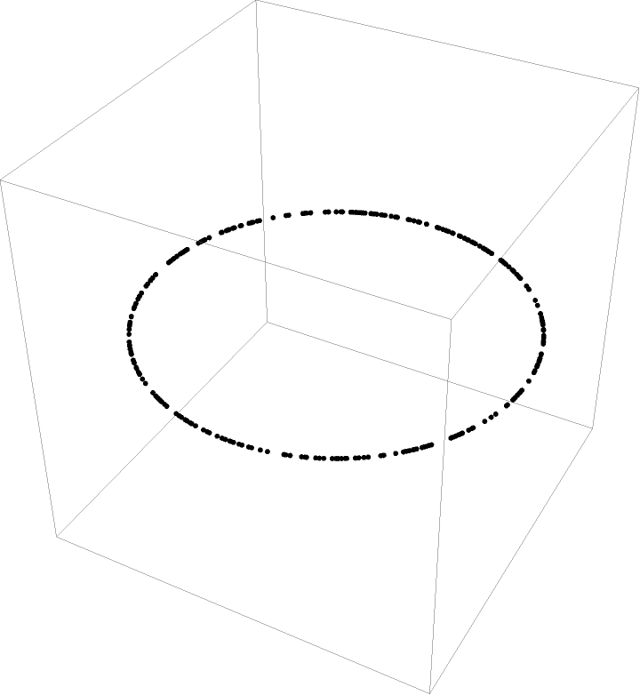
Closely approximate the radius of gyration of a given 2D region, for example, reproducing known quantities such as a hoop (unit circle):
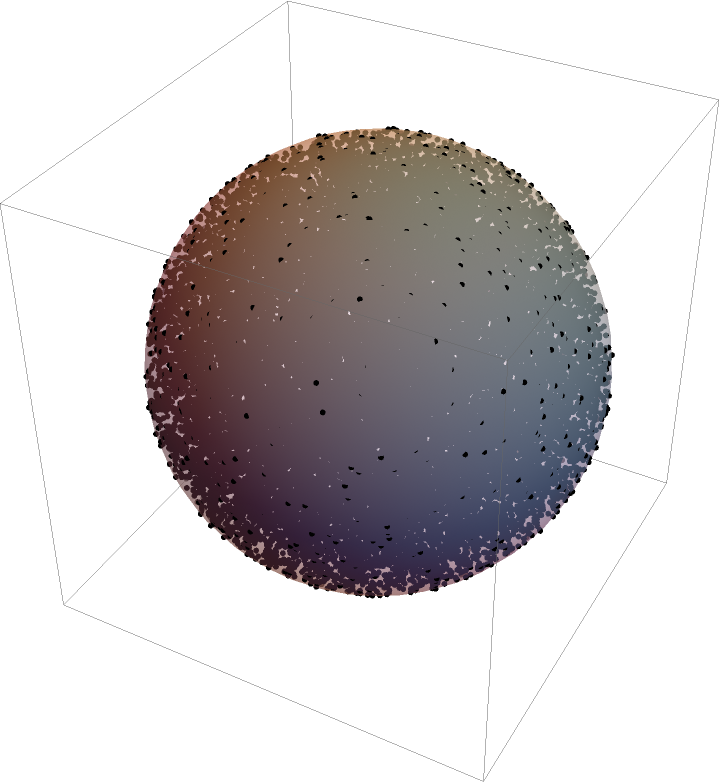
The same works for a hollow, 3D unit sphere:
The hollow sphere has a known radius of gyration Rg=R=1, which can be approximated (quite accurately, given the SpherePoints function):
The same works for a solid, 3D unit sphere, using ImplicitRegion:
The solid sphere has a known radius of gyration 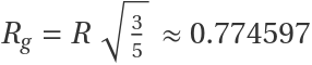 :
:
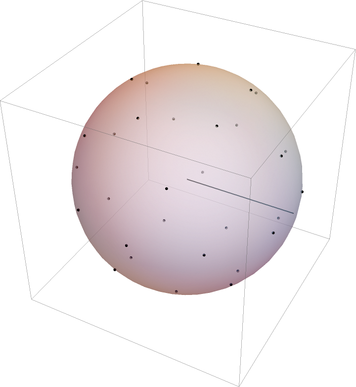
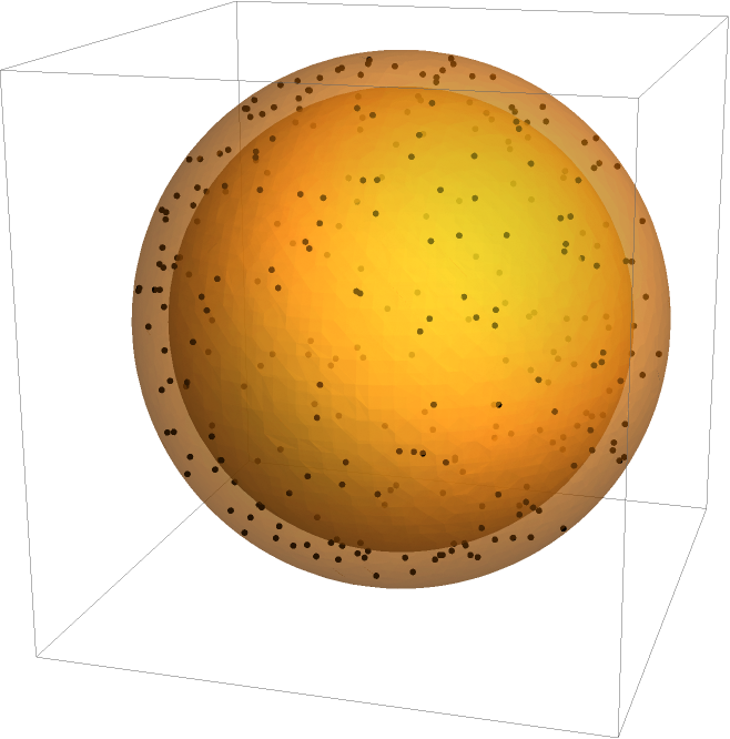
The intermediate result of a hollow spherical shell of a given thickness may also be estimated, using ImplicitRegion:
The radius of gyration may be estimated:
This result can be verified, in that it converges on the previous answer for the perfectly hollow unit sphere as thickness t→0:
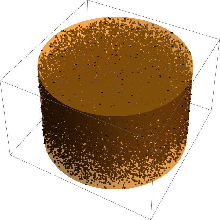
The same works for a solid, 3D cylinder, e.g. with unit radius and length, for which a Region may be defined from a pre-existing graphics primitive:
A solid cylinder has a known radius of gyration 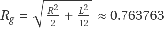 :
:
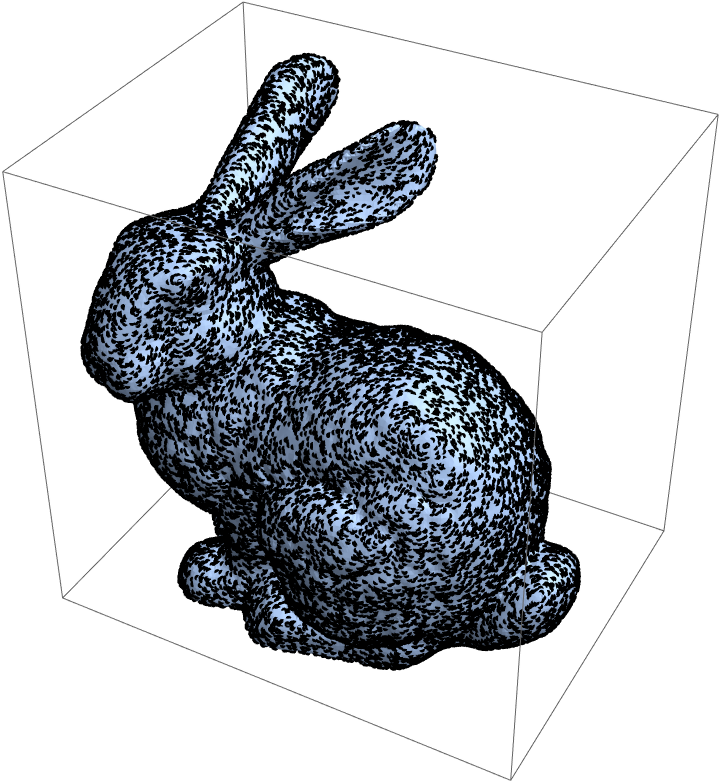
Estimate the radius of gyration of a rabbit from ExampleData:
Note that this is a hollow rabbit, so it is more relevant to the Easter chocolate shell version than a live rabbit:
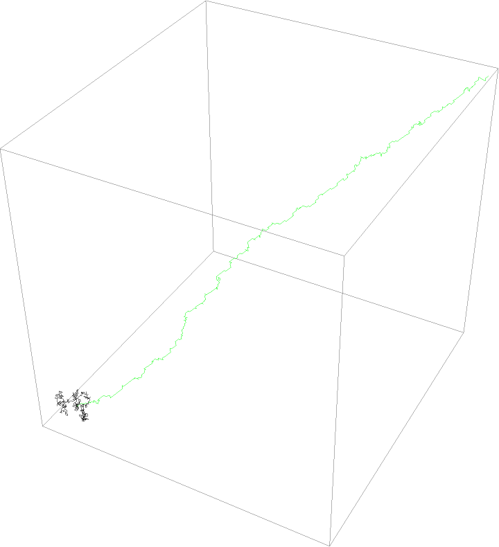
Shape metrics derived from the gyration tensor may be used to characterize the shape of a random walk. An unbiased random walk will generally have lower normalized asphericity than a biased random walk:
The unbiased walk (black) is much more spherically symmetric than the predominantly linear, biased random walk (green):
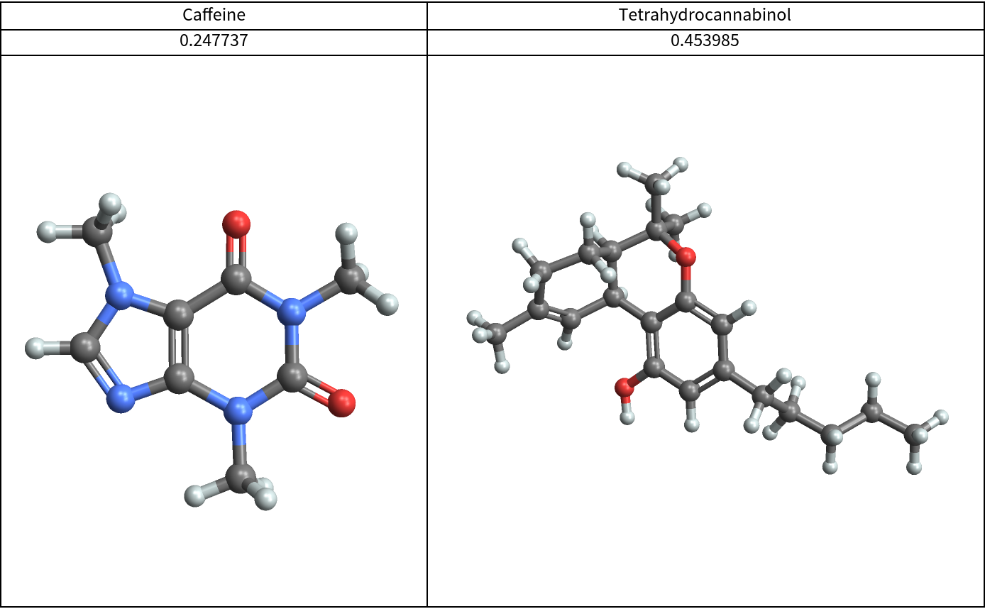
The relative anisotropy may be used to show that caffeine is a less linear molecule than THC:
![\[ScriptCapitalR] = ImplicitRegion[.75 <= x^2 + y^2 + z^2 <= 1, {x, y, z}];
coords = RandomPoint[\[ScriptCapitalR], 300];
Show[RegionPlot3D[\[ScriptCapitalR], PlotStyle -> Opacity[0.5], PlotPoints -> 50], Graphics3D[
Point[coords], {Thickness[0.005], Line[{{0, 0, 0}, +{1, 0, 0}}]}]]](https://www.wolframcloud.com/obj/resourcesystem/images/40d/40dee36b-fa82-4e85-89ea-e0104c9c392b/410c322a726f3b63.png)
![\[ScriptCapitalR] = ImplicitRegion[.99 <= x^2 + y^2 + z^2 <= 1, {x, y, z}];
coords = RandomPoint[\[ScriptCapitalR], 300];
ResourceFunction["GyrationTensor"][coords, "RadiusOfGyration"]](https://www.wolframcloud.com/obj/resourcesystem/images/40d/40dee36b-fa82-4e85-89ea-e0104c9c392b/373373c04d32cfe8.png)
![\[ScriptCapitalR] = Region@Cylinder[{{0, 0, 0}, {0, 0, 1}}];
coords = RandomPoint[\[ScriptCapitalR], 30000];
Show[RegionPlot3D[\[ScriptCapitalR], PlotStyle -> Opacity[0.5], PlotPoints -> 50], Graphics3D[
Point[coords], {Thickness[0.005], Line[{{0, 0, 0}, +{1, 0, 0}}]}], AspectRatio -> 1]](https://www.wolframcloud.com/obj/resourcesystem/images/40d/40dee36b-fa82-4e85-89ea-e0104c9c392b/03411bebde4a1892.png)
![\[ScriptCapitalR] = ExampleData[{"Geometry3D", "StanfordBunny"}, "Region"];
coords = RandomPoint[\[ScriptCapitalR], 30000];
Show[\[ScriptCapitalR], Graphics3D[{Point[coords]}], Boxed -> True]](https://www.wolframcloud.com/obj/resourcesystem/images/40d/40dee36b-fa82-4e85-89ea-e0104c9c392b/537c0e7e2d666f16.png)
![coordsUnbiased = N@Transpose[
RandomFunction[RandomWalkProcess[0.5], {0, 500}, 3][
"ValueList"]];
coordsBiased = N@Transpose[
RandomFunction[RandomWalkProcess[0.75], {0, 500}, 3]["ValueList"]];
Graphics3D[{Line[coordsUnbiased], {Green, Line[coordsBiased]}}, BoxRatios -> Automatic]](https://www.wolframcloud.com/obj/resourcesystem/images/40d/40dee36b-fa82-4e85-89ea-e0104c9c392b/5f56310576367cf0.png)
![Grid[Transpose[{#, ResourceFunction["GyrationTensor"][
QuantityMagnitude /@ ChemicalData[#, "AtomPositions"], "RelativeAnisotropy"], ChemicalData[#, "MoleculePlot"]} & /@ {"Caffeine", "Tetrahydrocannabinol"}], Frame -> All]](https://www.wolframcloud.com/obj/resourcesystem/images/40d/40dee36b-fa82-4e85-89ea-e0104c9c392b/0419908a0e32d52d.png)