Function Repository Resource:

DVectorField (1.0.1) current version: 1.1.0 »

Generate the tensor associated with the nth derivative of a vector field at a point

Contributed by: E. Chan-López, Víctor Castellanos, Héctor Argote Morales & Sjoerd Smit

ResourceFunction["DVectorField"][f,vars,p,n]

gives the tensor corresponding to the n^th derivative of a vector field f with respect to variables vars at a given point p.

Details

ResourceFunction["DVectorField"][f,vars, p, n] is a useful tool for computing the tensors associated with the Taylor approximations used in local bifurcation theory for nonlinear ordinary differential equations or nonlinear maps.

DvectorField[f,vars, p, n,"MultilinearFunction"] can be used to obtain multilinear functions associated with the tensors of each Taylor approximation.

DvectorField[f,vars, p, n,"MultilinearFunction"] generates new indexed symbols, such as x1, from the variables

of the vector field

, so once generated, preassigning values to these symbols should be avoided. These indexed symbols allow multilinear functions to be easily evaluated in calculations where they are required.

DvectorField[f,vars, p, n,"PureMultilinearFunction"] can be used to obtain multilinear functions associated with the tensors of each Taylor approximation using pure functions.

In typical usage, p will be an equilibrium point of the dynamical system f.

Examples

Basic Examples (2)

Use DVectorField with a 2D vector field:

In[1]:=

$MatrixForm@ ResourceFunction["DVectorField", ResourceVersion->"1.0.1"][{\[Alpha] - x y^2 + \[Beta] - \[Alpha] x \[Beta], (-y + x y^2) (\[Alpha] + \[Beta])}, {x, y}, {1, 2}, 2]$

Out[1]=

Use DVectorField with a 3D vector field:

In[2]:=

Out[2]=

Scope (3)

Use DVectorField with the Lorenz system to compute some multilinear functions:

In[3]:=

$Lorenz[{x_, y_, z_}][{\[Sigma]_, r_, \[Beta]_}] := {\[Sigma] (y - x), -x z + r x - y, x y - \[Beta] z}; X = {x, y, z}; \[Mu] = {\[Sigma], r, \[Beta]}; Column@Lorenz[X][\[Mu]]$

Out[6]=

Equilibrium points:

In[7]:=

$X0[{\[Sigma]_, r_, \[Beta]_}] := Evaluate[SolveValues[Lorenz[X][\[Mu]] == 0, X]] X1[{\[Sigma]_, r_, \[Beta]_}] = Part[X0[\[Mu]], 1]; X2[{\[Sigma]_, r_, \[Beta]_}] = Part[X0[\[Mu]], 2]; X3[{\[Sigma]_, r_, \[Beta]_}] = Part[X0[\[Mu]], 3]; Column@Map[Composition[MatrixForm, List], List[X1[\[Mu]], X2[\[Mu]], X3[\[Mu]]]]$

Out[11]=

Linear and bilinear functions for Lorenz system at the above equilibrium points:

In[12]:=

$Column[Map[ MatrixForm@ ResourceFunction["DVectorField"][Lorenz[X][\[Mu]], X, #, 1, "MultilinearFunction"] &, {X1[\[Mu]], X2[\[Mu]], X3[\[Mu]]}], Spacings -> 1]$

Out[12]=

In[13]:=

$Column[Map[ MatrixForm@ ResourceFunction["DVectorField"][Lorenz[X][\[Mu]], X, #, 2, "MultilinearFunction"] &, {X1[\[Mu]], X2[\[Mu]], X3[\[Mu]]}], Spacings -> 1]$

Out[13]=

Applications (37)

Hopf bifurcation analysis and first Lyapunov coefficient (3)

Compute the first Lyapunov coefficient for the Brusselator system:

In[14]:=

$Clear[X, \[Mu]]$

In[15]:=

$Brusselator[{x_, y_}][{\[Alpha]_, \[Beta]_}] := {\[Alpha] - (\[Beta] + 1) x + x^2 y, \[Beta] x - x^2 y} X = {x, y}; \[Mu] = {\[Alpha], \[Beta]}; Column@Brusselator[X][\[Mu]]$

Out[18]=

The equilibrium point:

In[19]:=

In[20]:=

$X0[{\[Alpha]_, \[Beta]_}] := Evaluate@SolveValues[Brusselator[X][\[Mu]] == 0, X][[1]] MatrixForm@List@X0[\[Mu]]$

Out[21]=

Assume α>0 fixed and take β as a bifurcation parameter to show that the system exhibits a supercritical Hopf bifurcation at X₀(α, β=β₀), where β₀=1+α².

The Jacobian matrix and its transpose:

In[22]:=

$J[{x_, y_}][{\[Alpha]_, \[Beta]_}] := Evaluate[D[Brusselator[X][\[Mu]], {X}]] MatrixForm@J[X][\[Mu]]$

Out[23]=

In[24]:=

$Jt[{x_, y_}][{\[Alpha]_, \[Beta]_}] := Evaluate[Transpose[J[X][\[Mu]]]] MatrixForm@Jt[X][\[Mu]]$

Out[25]=

Analyse the local stability with the resource function BialternateSum, with β as control parameter:

In[26]:=

$Reduce[Det[ResourceFunction["BialternateSum"][J[X0[\[Mu]]][\[Mu]]]] < 0 && \[Alpha] > 0 && \[Beta] > 0, \[Beta]]$

Out[26]=

The critical value of the Hopf bifurcation:

In[27]:=

$\[Beta]0 = Part[Normal[ SolveValues[ Det[ResourceFunction["BialternateSum"][J[X0[\[Mu]]][\[Mu]]]] == 0 && \[Alpha] > 0 && \[Beta] > 0, \[Beta]]], 1]$

Out[27]=

Then, the Brusselator system is locally asymptotically stable at X₀(μ) for β<β₀ and locally asymptotically unstable for β>β₀ (appears a stable limit cycle surrounded the unstable equilibrium point). We verify the previous conclusion by the transversality condition:

In[28]:=

$Factor[ReplaceAll[\[Beta] -> \[Beta]0][ 1/2 D[Det[ ResourceFunction["BialternateSum"][ J[X0[\[Mu]]][\[Mu]]]], \[Beta]]]]$

Out[28]=

The non-trivial equilibrium point at β=β₀:

In[29]:=

$X0\[Beta]0 = X0[{\[Alpha], \[Beta]0}]; MatrixForm@List@X0\[Beta]0$

Out[30]=

Shift the non-trivial equilibrium point to the origin:

In[31]:=

$Brusselator[{\[Xi]_, \[Eta]_}][\[Alpha]_] := Evaluate@ Collect[ReplaceAll[Thread[{x, y} -> {\[Xi], \[Eta]}]][ Brusselator[ X + X0\[Beta]0][{\[Alpha], \[Beta]0}]], {\[Xi], \[Eta]}, FullSimplify] X = {\[Xi], \[Eta]}; Column@Brusselator[X][\[Alpha]]$

Out[33]=

Verify that indeed the non-trivial equilibrium was shifted to the origin:

In[34]:=

$MatrixForm@List@Brusselator[{0, 0}][\[Alpha]]$

Out[34]=

The Jacobian matrix in the new state variables:

In[35]:=

In[36]:=

$J[{\[Xi]_, \[Eta]_}][\[Alpha]_] := Evaluate[ Collect[D[Brusselator[X][\[Alpha]], {X}], {\[Xi], \[Eta]}, FullSimplify]] MatrixForm@J[X][\[Alpha]]$

Out[37]=

The linear approximation at the origin and its transpose at β=1+α² and α=ω:

In[38]:=

In[39]:=

$\[Alpha] = \[Omega];$

In[40]:=

$J0[\[Omega]_] := Simplify@J[origin][\[Alpha]] MatrixForm@J0[\[Omega]]$

Out[41]=

In[42]:=

$J0T[\[Omega]_] := Simplify@Transpose[J[origin][\[Alpha]]] MatrixForm@J0T[\[Omega]]$

Out[43]=

In[44]:=

$MatrixForm@List@Simplify[Eigenvalues[J0[\[Omega]]]]$

Out[44]=

The critical eigenvectors q, , p, :

In[45]:=

$q = Eigenvectors[J0[\[Omega]]][[2]]; qc = ComplexExpand[Conjugate[q]]; pc = Eigenvectors[J0T[\[Omega]]][[1]]; p = ComplexExpand[Conjugate[pc]]; Row[Map[Composition[MatrixForm, List], {q, qc, p, pc}], " "]$

Out[49]=

The normalization 〈p_n,q〉=1

In[50]:=

Out[50]=

In[51]:=

$pn = 1/cn p; Row[Map[Composition[MatrixForm, List, Simplify], {pn, J0T[\[Alpha]] . pn - I \[Omega]*pn}], " "]$

Out[52]=

In[53]:=

Out[53]=

In[54]:=

$Row[Map[Composition[Simplify, MatrixForm, List], {J0[\[Alpha]] . q - I \[Omega]*q, J0[\[Alpha]] . qc + I \[Omega]*qc, J0T[\[Alpha]] . pn - I \[Omega]*pn, J0T[\[Alpha]] . pc + I \[Omega]*pc}], " "]$

Out[54]=

The third-order Taylor approximation for the polynomial system

Linear function:

In[55]:=

$AA[{\[Xi]1_, \[Eta]1_}][\[Alpha]_] := Evaluate[ ResourceFunction["DVectorField"][Brusselator[X][\[Alpha]], X, origin, 1, "MultilinearFunction"]] MatrixForm@AA[{\[Xi]1, \[Eta]1}][\[Omega]]$

Out[56]=

Bilinear function:

In[57]:=

$BB[{\[Xi]1_, \[Eta]1_}, {\[Xi]2_, \[Eta]2_}][\[Alpha]_] := Evaluate[ ResourceFunction["DVectorField"][Brusselator[X][\[Alpha]], X, origin, 2, "MultilinearFunction"]] MatrixForm@BB[{\[Xi]1, \[Eta]1}, {\[Xi]2, \[Eta]2}][\[Omega]]$

Out[58]=

Trilinear function:

In[59]:=

$CC[{\[Xi]1_, \[Eta]1_}, {\[Xi]2_, \[Eta]2_}, {\[Xi]3_, \[Eta]3_}][\[Alpha]_] := Evaluate[ ResourceFunction["DVectorField"][Brusselator[X][\[Alpha]], X, origin, 3, "MultilinearFunction"]] MatrixForm@ CC[{\[Xi]1, \[Eta]1}, {\[Xi]2, \[Eta]2}, {\[Xi]3, \[Eta]3}][\[Omega]]$

Out[60]=

Verify that the Taylor series expansion of the Brusselator system is correct:

In[61]:=

$MatrixForm@{FullSimplify[ Brusselator[X][\[Omega]] - (AA[{\[Xi], \[Eta]}][\[Omega]] + BB[{\[Xi], \[Eta]}, {\[Xi], \[Eta]}][\[Omega]]/2! + CC[{\[Xi], \[Eta]}, {\[Xi], \[Eta]}, {\[Xi], \[Eta]}][\[Omega]]/3!) /. {\[Xi] -> t \[Xi], \[Eta] -> t \[Eta]}]}$

Out[61]=

The first Lyapunov coefficient is given by:

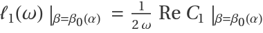
where

and h₂₀, h₁₁ are given by

h₂₀=(2 ⅈω 𝕀_2×2-AA)^-1BB(q,q), h₁₁=-AA^-1BB(q,q)

First, compute h₂₀, h₁₁ and C₁ as follows:

In[62]:=

$h20 = Simplify[(Inverse[ 2 I \[Omega]*IdentityMatrix[2] - J0[\[Omega]]]) . BB[q, q][\[Omega]]]; MatrixForm@List@h20$

Out[63]=

In[64]:=

$h11 = Simplify[-Inverse[J0[\[Omega]]] . BB[q, qc][\[Omega]]]; MatrixForm@List@h11$

Out[65]=

In[66]:=

$C1 = Simplify[ ComplexExpand[ pn . (CC[q, q, qc][\[Omega]] + BB[qc, h20][\[Omega]] + 2 BB[q, h11][\[Omega]])]]$

Out[66]=

Finally, compute the first Lyapunov coefficient:

In[67]:=

$Clear[\[Alpha]]$

In[68]:=

$\[Omega]0 = Normal[SolveValues[\[Alpha] == \[Omega] && \[Alpha] > 0 && \[Omega] > 0, \[Omega]]][[1]]$

Out[68]=

In[69]:=

$L1 = Factor@ ReplaceAll[\[Omega] -> \[Omega]0][ 1/(2 \[Omega]) ComplexExpand[Re[C1]]]$

Out[69]=

The first Lyapunov coefficient is clearly negative for all positive α. Thus, the Hopf bifurcation is nondegenerate and always supercritical.

Compute the first Lyapunov coefficient for the following predator-prey system:

In[70]:=

$Clear[X, \[Mu]]$

In[71]:=

$PredatorPrey[{x_, y_}][{c_, d_, r_, \[Alpha]_}] := {r x (1 - x) - ( c x y)/(x + \[Alpha]), -d y + (c x y)/(x + \[Alpha])} X = {x, y}; \[Mu] = {c, d, r, \[Alpha]}; Column[PredatorPrey[X][\[Mu]]]$

Out[74]=

The orbitally equivalent polynomial system:

In[75]:=

$PolynomialPredatorPrey[{x_, y_}][{c_, d_, r_, \[Alpha]_}] := Evaluate@ Map[Composition[Total, Factor, MonomialList[#, {x, y}] &, Expand, Factor, Times[#, x + \[Alpha]] &], PredatorPrey[X][\[Mu]]] Column@PolynomialPredatorPrey[X][\[Mu]]$

Out[76]=

The Jacobian matrix for the orbitally equivalent polynomial system:

In[77]:=

In[78]:=

$J[{x_, y_}][{c_, d_, r_, \[Alpha]_}] := Evaluate[Simplify@D[PolynomialPredatorPrey[X][\[Mu]], {X}]] MatrixForm@J[X][\[Mu]]$

Out[79]=

The non-trivial equilibrium point:

In[80]:=

In[81]:=

$X0[{c_, d_, r_, \[Alpha]_}] := Evaluate[ Simplify[ Normal[SolveValues[ PolynomialPredatorPrey[X][\[Mu]] == 0 && Reduce[Thread[Flatten[{X, \[Mu]}] > 0]], X][[1]]]]] MatrixForm@List@X0[\[Mu]]$

Out[82]=

The linear approximation at X₀(μ):

In[83]:=

In[84]:=

$J0[{c_, d_, r_, \[Alpha]_}] := Simplify@J[X0[\[Mu]]][\[Mu]] MatrixForm@J0[\[Mu]]$

Out[85]=

Analyse the local stability with the resource function BialternateSum, with α as control parameter:

In[86]:=

$Reduce[Det[ResourceFunction["BialternateSum"][J0[\[Mu]]]] < 0 && 0 < d < c && r > 0 && \[Alpha] > 0, \[Alpha]]$

Out[86]=

The critical value of the Hopf bifurcation:

In[87]:=

$\[Alpha]0 = Part[Normal[ SolveValues[ Det[ResourceFunction["BialternateSum"][J0[\[Mu]]]] == 0 && 0 < d < c && r > 0 && \[Alpha] > 0, \[Alpha]]], 1]$

Out[87]=

Then, the system is locally asymptotically stable for α>α₀ and locally asymptotically unstable for α<α₀ (with c>d), and can be confirmed by the transversality condition:

In[88]:=

$Factor[ReplaceAll[\[Alpha] -> \[Alpha]0][ 1/2 D[Det[ ResourceFunction["BialternateSum"][J0[\[Mu]]]], \[Alpha]]]]$

Out[88]=

The non-trivial equilibrium point at α=α₀:

In[89]:=

$X0\[Alpha]0 = Simplify[X0[{c, d, r, \[Alpha]0}]]; MatrixForm@List@X0\[Alpha]0$

Out[90]=

Shift the non-trivial equilibrium point to the origin:

In[91]:=

$PolynomialPredatorPrey[{\[Xi]_, \[Eta]_}][{c_, d_, r_}] := Evaluate@ Map[Composition[Total, Collect[#, {\[Xi], \[Eta]}, FullSimplify] &, MonomialList[#, {\[Xi], \[Eta]}] &], ReplaceAll[Thread[{x, y} -> {\[Xi], \[Eta]}]][ PolynomialPredatorPrey[X + X0\[Alpha]0][{c, d, r, \[Alpha]0}]]] X = {\[Xi], \[Eta]}; \[Mu]3 = {c, d, r}; Column[PolynomialPredatorPrey[X][\[Mu]3]]$

Out[92]=

Verify that indeed the non-trivial equilibrium was shifted to the origin:

In[93]:=

$MatrixForm[{Simplify[ ReplaceAll[{\[Xi] -> -Part[X0\[Alpha]0, 1], \[Eta] -> -Part[ X0\[Alpha]0, 2]}][PolynomialPredatorPrey[X][\[Mu]3]]]}]$

Out[93]=

The Jacobian matrix in the new state variables:

In[94]:=

$J[{\[Xi]_, \[Eta]_}][{c_, d_, r_}] := Evaluate[ Collect[D[PolynomialPredatorPrey[X][\[Mu]3], {X}], {\[Xi], \[Eta]}, FullSimplify]] MatrixForm@J[X][\[Mu]3]$

Out[95]=

The linear approximation at the origin and at 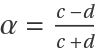and :

In[96]:=

In[97]:=

In[98]:=

$r0 = ((c + d)^3 \[Omega]^2)/(c^2 (c - d) d);$

In[99]:=

$\[Mu]2 = {c, d};$

In[100]:=

In[101]:=

$J0[{c_, d_}] := Simplify@J[origin][{c, d, r0}] MatrixForm@J0[\[Mu]2]$

Out[89]=

In[102]:=

In[103]:=

$J0T[{c_, d_}] := Simplify@Transpose[J[origin][{c, d, r0}]] MatrixForm@J0T[\[Mu]2]$

Out[104]=

In[105]:=

$MatrixForm@List@Simplify[Eigenvalues[J0[\[Mu]2]]]$

Out[105]=

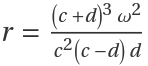The critical eigenvectors q, , p, :

In[106]:=

In[107]:=

$q = -I \[Omega] (c + d)*Eigenvectors[J0[\[Mu]2]][[2]]; qc = ComplexExpand[Conjugate[q]]; pc = -I c d*Eigenvectors[J0T[\[Mu]2]][[1]]; p = ComplexExpand[Conjugate[pc]]; Row[Map[Composition[MatrixForm, List], {q, qc, p, pc}], " "]$

Out[111]=

The normalization 〈p_n,q〉=1

In[112]:=

In[113]:=

Out[113]=

In[114]:=

In[115]:=

$pn = 1/cn p; Row[Map[Composition[MatrixForm, List, Simplify], {pn, J0T[\[Mu]2] . pn - I \[Omega]*pn}], " "]$

Out[116]=

In[117]:=

Out[117]=

In[118]:=

$Row[Map[Composition[MatrixForm, List, Simplify], {J0[\[Mu]2] . q - I \[Omega]*q, J0[\[Mu]2] . qc + I \[Omega]*qc, J0T[\[Mu]2] . pn - I \[Omega]*pn, J0T[\[Mu]2] . pc + I \[Omega]*pc}], " "]$

Out[118]=

The third-order Taylor approximation for the polynomial system

Linear function:

In[119]:=

In[120]:=

$AA[{\[Xi]1_, \[Eta]1_}][{c_, d_, r_}] := Evaluate[ ResourceFunction["DVectorField"][PolynomialPredatorPrey[X][\[Mu]3], X, origin, 1, "MultilinearFunction"]] MatrixForm@AA[{\[Xi]1, \[Eta]1}][\[Mu]3]$

Out[121]=

Bilinear function:

In[122]:=

In[123]:=

$BB[{\[Xi]1_, \[Eta]1_}, {\[Xi]2_, \[Eta]2_}][{c_, d_, r_}] := Evaluate[ ResourceFunction["DVectorField"][PolynomialPredatorPrey[X][\[Mu]3], X, origin, 2, "MultilinearFunction"]] MatrixForm@BB[{\[Xi]1, \[Eta]1}, {\[Xi]2, \[Eta]2}][\[Mu]3]$

Out[124]=

Trilinear function:

In[125]:=

In[126]:=

$CC[{\[Xi]1_, \[Eta]1_}, {\[Xi]2_, \[Eta]2_}, {\[Xi]3_, \[Eta]3_}][{c_, d_, r_}] := Evaluate[ ResourceFunction["DVectorField"][PolynomialPredatorPrey[X][\[Mu]3], X, origin, 3, "MultilinearFunction"]] MatrixForm@ CC[{\[Xi]1, \[Eta]1}, {\[Xi]2, \[Eta]2}, {\[Xi]3, \[Eta]3}][\[Mu]3]$

Out[127]=

Verify that the Taylor series expansion of the polynomial system is correct:

In[128]:=

$MatrixForm@{FullSimplify[ PolynomialPredatorPrey[X][{c, d, r0}] - (AA[{\[Xi], \[Eta]}][{c, d, r0}] + BB[{\[Xi], \[Eta]}, {\[Xi], \[Eta]}][{c, d, r0}]/2! + CC[{\[Xi], \[Eta]}, {\[Xi], \[Eta]}, {\[Xi], \[Eta]}][{c, d, r0}]/3!) /. {\[Xi] -> t \[Xi], \[Eta] -> t \[Eta]}]}$

Out[128]=

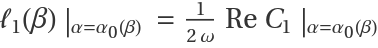
The first Lyapunov coefficient is given by:

where

and h₂₀, h₁₁ are given by

h₂₀=(2 ⅈω 𝕀_2×2-AA)^-1BB(q,q), h₁₁=-AA^-1BB(q,q)

First, compute h₂₀, h₁₁ and C₁ as follows:

In[129]:=

In[130]:=

$h20 = Simplify[(Inverse[ 2 I \[Omega]*IdentityMatrix[2] - J0[\[Mu]2]]) . BB[q, q][\[Mu]3]]; MatrixForm@List@h20$

Out[131]=

In[132]:=

In[133]:=

$h11 = Simplify[-Inverse[J0[\[Mu]2]] . BB[q, qc][\[Mu]3]]; MatrixForm@List@h11$

Out[134]=

In[135]:=

In[136]:=

$C1 = Simplify[ ComplexExpand[ pn . (CC[q, q, qc][\[Mu]3] + BB[qc, h20][\[Mu]3] + 2 BB[q, h11][\[Mu]3])]]$

Out[136]=

Finally, we compute the first Lyapunov coefficient:

In[137]:=

In[138]:=

$L1 = FullSimplify[1/(2 \[Omega]) ComplexExpand[Re[C1]]]$

Out[138]=

Clearly, the first Lyapunov coefficient is strictly negative for all combinations of the fixed parameters. Therefore, a unique limit cycle emerges from the non-trivial equilibrium via Hopf bifurcation for α<α₀.

Compute the first Lyapunov coefficient for the following nonlinear feedback-control system of Lur'e type:

In[139]:=

$Clear[X, \[Mu]]$

In[140]:=

$Lure[{x_, y_, z_}][{\[Alpha]_, \[Beta]_}] := {y, z, -x + x^2 - \[Beta] y - \[Alpha] z}; X = {x, y, z}; \[Mu] = {\[Alpha], \[Beta]}; Column@Lure[X][\[Mu]]$

Out[143]=

For all values of (α>0,β>0), the Lur'e system has two equilibria, the origin and (1,0,0). At the origin, this system exhibits a supercritical Hopf bifurcation when α=α₀, where :

In[144]:=

In[145]:=

$X0[{\[Alpha]_, \[Beta]_}] := Evaluate[SolveValues[Lure[X][\[Mu]] == 0, X]] Row@Map[Composition[MatrixForm, List], X0[\[Mu]]]$

Out[146]=

The Jacobian matrix and its transpose:

In[147]:=

In[148]:=

$J[{x_, y_, z_}][{\[Alpha]_, \[Beta]_}] := Evaluate[D[Lure[X][\[Mu]], {X}]] MatrixForm@J[X][\[Mu]]$

Out[149]=

In[150]:=

In[151]:=

$Jt[{x_, y_, z_}][{\[Alpha]_, \[Beta]_}] := Evaluate[Transpose[J[X][\[Mu]]]] MatrixForm@Jt[X][\[Mu]]$

Out[152]=

Analyse the local stability with the resource function BialternateSum, with β as control parameter:

In[153]:=

$Reduce[Det[ ResourceFunction["BialternateSum"][ Evaluate@J[X0[\[Mu]][[1]]][\[Mu]]]] < 0 && \[Alpha] > 0 && \[Beta] > 0, \[Alpha]]$

Out[153]=

The critical value of the Hopf bifurcation:

In[154]:=

$Clear[\[Alpha]0]$

In[155]:=

$\[Alpha]0 = Part[Normal[ SolveValues[ Det[ResourceFunction["BialternateSum"][ J[X0[\[Mu]][[1]]][\[Mu]]]] == 0 && \[Alpha] > 0 && \[Beta] > 0, \[Alpha]]], 1]$

Out[155]=

Then, the Lur'e system is locally asymptotically stable at X₀(μ) for α>α₀ and locally asymptotically unstable for α<α₀ (appears a stable limit cycle surrounded the unstable equilibrium point). We verify the previous conclusion by the transversality condition:

In[156]:=

$Factor[ReplaceAll[\[Alpha] -> \[Alpha]0][ 1/2 D[Det[ ResourceFunction["BialternateSum"][ J[X0[\[Mu]][[1]]][\[Mu]]]], \[Alpha]]]]$

Out[156]=

The linear approximation at the origin and its transpose at and β=ω²:

In[157]:=

$\[Beta] = \[Omega]^2;$

In[158]:=

In[159]:=

$J0[\[Omega]_] := Simplify@J[X0[{\[Alpha]0, \[Beta]}][[1]]][{\[Alpha]0, \[Beta]}] MatrixForm[J0[\[Omega]]]$

Out[160]=

In[161]:=

In[162]:=

$J0T[\[Omega]_] := Simplify@Transpose[J0[\[Omega]]] MatrixForm[J0T[\[Omega]]]$

Out[163]=

In[164]:=

$MatrixForm@List@Simplify[Eigenvalues[J0[\[Omega]]]]$

Out[164]=

The critical eigenvectors q, , p, :

In[165]:=

In[166]:=

$q = -\[Omega]^2*Eigenvectors[J0[\[Omega]]][[3]]; qc = ComplexExpand[Conjugate[q]]; p = -\[Omega]^2*Eigenvectors[J0T[\[Omega]]][[2]] // Expand; pc = ComplexExpand[Conjugate[p]]; Row[Map[Composition[MatrixForm, List], {q, qc, p, pc}], " "]$

Out[170]=

The normalization 〈p_n,q〉=1

In[171]:=

In[172]:=

Out[172]=

In[173]:=

In[174]:=

$pn = Map[Total, MapAt[Composition[FullSimplify, Times[#, I] &], ComplexExpand@ReIm[1/cn pc], {All, 2}]]; Row[Map[Composition[MatrixForm, List, Simplify], {pn, J0T[\[Omega]] . pn - I \[Omega]*pn}], " "]$

Out[175]=

In[176]:=

Out[176]=

In[177]:=

$Row[Map[Composition[Simplify, MatrixForm, List], {J0[\[Alpha]] . q - I \[Omega]*q, J0[\[Alpha]] . qc + I \[Omega]*qc, J0T[\[Alpha]] . p + I \[Omega]*p, J0T[\[Alpha]] . pn - I \[Omega]*pn}], " "]$

Out[177]=

The third-order Taylor approximation for the polynomial system

Linear function:

In[178]:=

In[179]:=

$AA[{x1_, y1_, z1_}][\[Omega]_] := Evaluate[ ResourceFunction["DVectorField"][Lure[X][{\[Alpha]0, \[Beta]}], X, X0[{\[Alpha]0, \[Beta]}][[1]], 1, "MultilinearFunction"]] MatrixForm@AA[{x1, y1, z1}][\[Omega]]$

Out[180]=

Bilinear function:

In[181]:=

In[182]:=

$BB[{x1_, y1_, \[FormalZ]1_}, {x2_, y2_, z2_}][\[Omega]_] := Evaluate[ ResourceFunction["DVectorField"][Lure[X][{\[Alpha]0, \[Beta]}], X, X0[{\[Alpha]0, \[Beta]}][[1]], 2, "MultilinearFunction"]] MatrixForm@BB[{x1, y1, z1}, {x2, y2, z2}][\[Omega]]$

Out[183]=

Trilinear function:

In[184]:=

In[185]:=

$CC[{x1_, y1_, z1_}, {x2_, y2_, z2_}, {x3_, y3_, z3_}][\[Omega]_] := Evaluate[ ResourceFunction["DVectorField"][Lure[X][{\[Alpha]0, \[Beta]}], X, X0[{\[Alpha]0, \[Beta]}][[1]], 3, "MultilinearFunction"]] MatrixForm@CC[{x1, y1, z1}, {x2, y2, z2}, {x3, y3, z3}][\[Omega]]$

Out[186]=

We verify that the Taylor series expansion of the Lur'e system is correct:

In[187]:=

$MatrixForm@{FullSimplify[ Lure[X][{\[Alpha]0, \[Beta]}] - (AA[X][\[Omega]] + BB[X, X][\[Omega]]/2! + CC[X, X, X][\[Omega]]/3!) /. {x -> t x, y -> t y, z -> t z}]}$

Out[187]=

The first Lyapunov coefficient is given by:

where

and h₂₀, h₁₁ are given by

h₂₀=(2 ⅈω 𝕀_3×3-AA)^-1BB(q,q), h₁₁=-AA^-1BB(q,q)

First, compute h₂₀, h₁₁ and C₁

In[188]:=

In[189]:=

$h20 = (Inverse[2 I \[Omega]*IdentityMatrix[3] - J0[\[Omega]]]) . BB[q, q][\[Omega]]; MatrixForm[{h20}]$

Out[190]=

In[191]:=

In[192]:=

$h11 = -Inverse[J0[\[Omega]]] . BB[q, qc][\[Omega]]; MatrixForm[{h11}]$

Out[193]=

In[194]:=

In[195]:=

$C1 = ComplexExpand[ pn . (CC[q, q, qc][\[Omega]] + BB[qc, h20][\[Omega]] + 2 BB[q, h11][\[Omega]])]$

Out[195]=

Finally, compute the first Lyapunov coefficient:

In[196]:=

$Clear[\[Omega]0, \[Beta]]$

In[197]:=

$\[Omega]0 = Normal[SolveValues[\[Beta] == \[Omega]^2 && \[Beta] > 0 && \[Omega] > 0, \[Omega]]][[1]]$

Out[197]=

In[198]:=

In[199]:=

$L1 = Factor[ 1/(2 \[Omega]) ComplexExpand[Re[C1]] /. \[Omega] -> \[Omega]0]$

Out[199]=

In[200]:=

Simplify@
Numerator[L1]/(Times[#[[1]], #[[2]]] &@
MapAt[Composition[Simplify, Times[#[[1]], #[[2]]] &], List[Extract[FactorList[Denominator[L1]][[All, 1]], {{2}, {3}}], Extract[FactorList[Denominator[L1]][[All, 1]], {4}]], {1}])

Out[200]=

The first Lyapunov coefficient is strictly negative for all positive β. Thus, the Hopf bifurcation is nondegenerate and always supercritical.

Neimark-Sacker bifurcation analysis and first Lyapunov coefficient (19)

The recurrence equation 𝓊_k+1=𝓇 𝓊_k+1(1-𝓊_k-1) is simple population dynamical model, where 𝓊_k depict for the density of a population at time k, and 𝓇 is a growth rate. Introducing 𝓊_k=𝓊_k-1, the above equation can be rewritten as

𝓊_k+1=𝓇 𝓊_k(1-𝓋_k), 𝓋_k+1= 𝓋_k,

which, in turn, defines the following two-dimensional discrete-time dynamical system

Define the discrete-time dynamical system (1) as follows:

In[201]:=

In[202]:=

$LogisticMap[{x_, y_}][r_] := {r x (1 - y), x} X = {x, y}; Column@LogisticMap[X][r]$

Out[204]=

Jacobian matrix:

In[205]:=

In[206]:=

$J[{x_, y_}][r_] := Evaluate[Simplify@D[LogisticMap[X][r], {X}]] MatrixForm@J[X][r]$

Out[207]=

The non-trivial fixed point:

In[208]:=

In[209]:=

Out[210]=

The linear approximation at X₀(r):

In[211]:=

Out[212]=

The eigenvalues of the linear approximation A:

In[213]:=

Out[213]=

For 𝓇>5/4 the eigenvalues are complex, so the following shift is made in the growth rate 𝓇 to handle this restriction, and then the eigenvalues of Aare computed again:

In[214]:=

In[215]:=

Out[215]=

In[216]:=

$\[Zeta] = Refine[Eigenvalues[A[rc]], Assumptions -> r0 > 0]; MatrixForm@List@\[Zeta]$

Out[217]=

The value 𝓇₀ where the fixed point X₀(𝓇₀) loses its stability, giving rise to a Neimark-Sacker bifurcation, is given by:

In[218]:=

$r0ns = SolveValues[(\[Zeta][[1]]*\[Zeta][[2]]) == 1, r0][[1]]$

Out[218]=

Therefore, the fixed point X₀(𝓇₀) loses its stability at 𝓇=2 as verified below:

In[219]:=

Out[219]=

The linear approximation A(𝓇) at the critical bifurcation value 𝓇=2 and its transpose:

In[220]:=

Out[221]=

In[222]:=

Out[223]=

The critical multipliers are given by:

In[224]:=

Out[224]=

In[225]:=

$\[Zeta]1 = E^(I \[Theta]0); \[Zeta]2 = E^(-I \[Theta]0); \[Theta]0 = ArcTan[Sqrt[3]];$

The transversality condition:

In[226]:=

Out[226]=

The nondegeneracy condition:

ζⁿ≠1, for n=1,2,3,4.

In[227]:=

$MatrixForm@List@ComplexExpand@Array[ToExpression["\[Zeta]1"]^# &, 4]$

Out[227]=

The critical eigenvectors q, , p, :

In[228]:=

In[229]:=

q = ComplexExpand@Eigenvectors[A0][[1]];
qc = ComplexExpand@Eigenvectors[A0][[2]];
p = ComplexExpand@Eigenvectors[A0T][[1]];
pc = ComplexExpand@Eigenvectors[A0T][[2]];
Row[Map[Composition[MatrixForm, List], {q, qc, p, pc}], " "]

Out[233]=

The normalization 〈p_n,q〉=1

In[234]:=

In[235]:=

Out[235]=

In[236]:=

In[237]:=

Out[238]=

In[239]:=

$Row[Map[Composition[MatrixForm, List, ComplexExpand], {pn, A0T . pn - \[Zeta]1*pn}], " "]$

Out[239]=

In[240]:=

Out[240]=

In[241]:=

$Row[Map[Composition[MatrixForm, List, Simplify], {A0 . q - \[Zeta]1*q, A0 . qc - \[Zeta]2*qc, A0T . pn - \[Zeta]1*pn, A0T . pc - \[Zeta]2*pc}], " "]$

Out[241]=

The bilinear and trilinear forms to compute the first Lyapunov coefficient:

In[242]:=

In[243]:=

$BB[{x1_, y1_}, {x2_, y2_}][r_] := Evaluate[ ResourceFunction["DVectorField"][LogisticMap[X][r], X, X0[r], 2, "MultilinearFunction"]] MatrixForm@BB[{x1, y1}, {x2, y2}][r]$

Out[244]=

In[245]:=

In[246]:=

$CC[{x1_, y1_}, {x2_, y2_}, {x3_, y3_}][r_] := Evaluate[ ResourceFunction["DVectorField"][LogisticMap[X][r], X, X0[r], 3, "MultilinearFunction"]] MatrixForm@CC[{x1, y1}, {x2, y2}, {x3, y3}][r]$

Out[247]=

The first Lyapunov coefficient (additional nondegeneracy condition) is given by

Finally, compute the first Lyapunov coefficient:

In[248]:=

Out[249]=

In[250]:=

$S2 = ComplexExpand[ Inverse[\[Zeta]1^2*IdentityMatrix[2] - A0] . BB[q, q][2]]; MatrixForm@List@S2$

Out[251]=

In[252]:=

$d0 = 1/2* Re[\[Zeta]2*(pn . CC[q, q, qc][2] + 2*pn . BB[q, S1][2] + pn . BB[qc, S2][2])]$

Out[252]=

Therefore, a unique and stable closed invariant curve bifurcates from the non-trivial fixed point X₀(𝓇) for 𝓇>2.

Quadratic coefficients of the normal form for Bogdanov-Takens bifurcation (15)

Compute the quadratic coefficients of the Bogdanov-Takens bifurcation normal form for a predator-prey model with non-linear predator reproduction and prey competition:

In[253]:=

$Clear[PredatorPrey, X, \[Mu]]$

In[254]:=

$PredatorPrey[{x_, y_}][{\[Gamma]_, \[Epsilon]_, n_}] := Evaluate@{x (1 - y) - \[Epsilon] x^2, -\[Gamma] y + (y/(n + y)) x y} X = {x, y}; \[Mu] = {\[Gamma], \[Epsilon], n}; Column[PredatorPrey[X][\[Mu]]]$

Out[105]=

The Jacobian matrix:

In[255]:=

$J[{x_, y_}][{\[Gamma]_, \[Epsilon]_, n_}] := Evaluate[Simplify[D[PredatorPrey[X][\[Mu]], {X}]]] MatrixForm@J[X][\[Mu]]$

Out[59]=

Look for the Bogdanov-Takens point:

In[256]:=

$Factor@Reduce[ PredatorPrey[X][\[Mu]] == 0 && Tr[J[X][\[Mu]]] == 0 && Det[J[X][\[Mu]]] == 0 && (And @@ Thread[Variables[PredatorPrey[X][\[Mu]]] > 0]), {x, \[Gamma], \[Epsilon], n}, Backsubstitution -> True]$

Out[256]=

To explicitly handle constraint , apply the following shift to get the Bogdanov-Takens point:

In[257]:=

$BTPoint = First@Factor@(SolveValues[ PredatorPrey[X][\[Mu]] == 0 && Tr[J[X][\[Mu]]] == 0 && Det[J[X][\[Mu]]] == 0, {x, \[Gamma], \[Epsilon], n}] /. y -> \[Zeta]0/(2 (1 + \[Zeta]0)))$

Out[257]=

With the above shift in the predator population, the equilibrium point of coexistence and the critical value of bifurcation are as follows:

In[258]:=

In[259]:=

$X0[\[Zeta]0_] := Evaluate[{BTPoint[[1]], \[Zeta]0/(2 (1 + \[Zeta]0))}] MatrixForm@List@X0[\[Zeta]0]$

Out[258]=

In[260]:=

$\[Mu]0[\[Zeta]0_] := BTPoint[[2 ;; 4]] MatrixForm@List@\[Mu]0[\[Zeta]0]$

Out[261]=

The linear approximation at x₀(ζ₀):

In[262]:=

In[263]:=

$J0[\[Zeta]0_] := Simplify@(J[X0[\[Zeta]0]][\[Mu]0[\[Zeta]0]]) MatrixForm@J0[\[Zeta]0]$

Out[67]=

Verify that J₀(ζ₀) has a pair of null eigenvalues:

In[264]:=

$MatrixForm@List@Eigenvalues[J0[\[Zeta]0]]$

Out[264]=

The critical right eigenvectors q₀ and q₁:

In[265]:=

$q0 = Factor[Part[NullSpace[J0[\[Zeta]0]], 1]]; MatrixForm@List@q0$

Out[70]=

In[266]:=

$q1 = Simplify@ ReplaceAll[r1 -> 0][{r1, Part[SolveValues[J0[\[Zeta]0] . {r1, r2} == q0, r2], 1]}]; MatrixForm@List@q1$

Out[267]=

Verify the conditions 〈J₀(ζ₀),q₀〉=0 y 〈J₀(ζ₀),q₁〉=q₀

In[268]:=

$Column[Map[ Composition[MatrixForm, List, Simplify], {J0[\[Zeta]0] . q0, J0[\[Zeta]0] . q1 - IdentityMatrix[2] . q0}], Spacings -> 1]$

Out[268]=

The transition matrix Q with the critical right eigenvectors:

In[269]:=

Out[75]=

The critical left eigenvectors p₀ and p₁:

In[270]:=

Out[77]=

In[271]:=

Out[272]=

In[273]:=

Out[94]=

Verify the conditions 〈J₀(ζ₀)^T,p₁〉=0 y 〈J₀(ζ₀)^T,p₀〉=p₁

In[274]:=

$Column[Map[ Composition[MatrixForm, List, Simplify], {Transpose[J0[\[Zeta]0]] . p1, Transpose[J0[\[Zeta]0]] . p0 - IdentityMatrix[2] . p1}], Spacings -> 1]$

Out[274]=

Finally, verify the conditions 〈q₀,p₀〉=〈q₁,p₁〉=1 y 〈q₀,p₁〉=〈q₁,p₀〉=0 and that the matrix J₀(ζ₀) is similar to a simple Jordan block:

In[275]:=

Out[275]=

In[276]:=

$MatrixForm@Factor[QI . J0[\[Zeta]0] . Q]$

Out[276]=

The quadratic coefficients, involved in the nondegeneracy condition, can be computed in the following two ways:

In[277]:=

In[278]:=

$BB[{x1_, y1_}, {x2_, y2_}][\[Zeta]0_] := Evaluate[ ResourceFunction["DVectorField"][PredatorPrey[X][\[Mu]0[\[Zeta]0]], X, X0[\[Zeta]0], 2, "MultilinearFunction"]] MatrixForm@BB[{x1, y1}, {x2, y2}][\[Zeta]0]$

Out[112]=

In[279]:=

$a = Simplify[1/2 p1 . BB[q0, q0][\[Zeta]0]]$

Out[279]=

In[280]:=

$b = Simplify[p0 . BB[q0, q0][\[Zeta]0] + p1 . BB[q0, q1][\[Zeta]0]]$

Out[280]=

In[281]:=

In[282]:=

$D20[\[Zeta]0_] := Evaluate[ Simplify[ ResourceFunction["DVectorField"][PredatorPrey[X][\[Mu]0[\[Zeta]0]], X, X0[\[Zeta]0], 2]]] MatrixForm@D20[\[Zeta]0]$

Out[283]=

In[284]:=

$a = Factor@(1/2 q0 . (p1 . D20[\[Zeta]0] . q0))$

Out[284]=

In[285]:=

$b = Factor@((q0 . (p0 . D20[\[Zeta]0])) . q0 + (q0 . (p1 . D20[\[Zeta]0])) . q1)$

Out[285]=

The Bogdanov-Takens bifurcation in this case is non-degenerate when ζ₀!=2 and the unique point of degeneracy is:

In[286]:=

$Append[List[Thread[{x, y} -> X0[2]]], Thread[{\[Gamma], \[Epsilon], n} -> ReplaceAll[\[Zeta]0 -> 2][\[Mu]0[\[Zeta]0]]]]$

Out[286]=

Properties and Relations (1)

Use DVectorField with the resource function SymbolToSubscript:

In[287]:=

$MatrixForm@ ResourceFunction["DVectorField", ResourceVersion->"1.0.1"][{-x y^2 z + \[Alpha] - \[Beta] x, -y w + x y^2, x y z + w^2, x y z^2 w^3}, {x, y, z, w}, {1, 1, 0, 1}, 3, "MultilinearFunction"]$

Out[287]=

In[288]:=

Out[288]=

Possible Issues (3)

Using the option "MultilinearFunction", DVectorField creates new indexed and unprotected variables from the original ones. This can be problematic if the “new” variables were previously assigned, as shown below:

In[289]:=

In[290]:=

$MatrixForm@ ResourceFunction["DVectorField", ResourceVersion->"1.0.1"][{\[Alpha] - x y^2 + \[Beta] - \[Alpha] x \[Beta], (-y + x y^2) (\[Alpha] + \[Beta])}, {x, y}, {1, 2}, 3, "MultilinearFunction"]$

Out[290]=

To handle this possible problem, it is recommended to avoid preassigning the unprotected variables generated by DVectorField. In this way, if in the previous example we clean the assigned variables, we obtain the correct trilinear function:

In[291]:=

In[292]:=

Out[292]=

When we want to copy our results to LaTeX code, the"MultilinearFunction" option is very useful in combination with the resource function SymbolToSubscript, but we must always keep a strict control of the new symbols generated so as not to pre-assign values to them.

If we are not interested in copying expressions to LaTeX code and want to avoid conflicts with unprotected symbols, DVectorField has the "PureMultilinearFunction" option to work with pure functions, for example:

In[293]:=

$D20[{{x1_, y1_}, {x2_, y2_}}] = ResourceFunction["DVectorField"][{x - y^2, 2 y/x}, {x, y}, {1, 2}, 2, "MultilinearFunction"]$

Out[293]=

In[294]:=

$D21 = ResourceFunction["DVectorField", ResourceVersion->"1.0.1"][{x - y^2, 2 y/x}, {x, y}, {1, 2}, 2, "PureMultilinearFunction"]$

Out[294]=

In[295]:=

Out[295]=

Publisher

Ramón Eduardo Chan López

Version History

1.1.0 – 02 October 2023
1.0.1 – 07 November 2022
1.0.0 – 14 October 2022

Source Metadata

Citation:
- Asada, T., & Ishikawa, T. (2007). Time and space in economics. Springer Science & Business Media.
- Fuller, A. T. (1968). Conditions for a matrix to have only characteristic roots with negative real parts. Journal of Mathematical Analysis and Applications, 23(1), 71-98. DOI: 10.1016/0022-247X(68)90116-9
- Govaerts, W. J. (2000). Numerical methods for bifurcations of dynamical equilibria. Society for Industrial and Applied Mathematics.
- Guckenheimer, J., Myers, M., & Sturmfels, B. (1997). Computing Hopf bifurcations I. SIAM Journal on Numerical Analysis, 34(1), 1-21. DOI: 10.1137/S0036142993253461
- Jury, E., & Gutman, S. (1975). On the stability of the A matrix inside the unit circle. IEEE Transactions on Automatic Control, 20(4), 533-535. DOI: 10.1109/TAC.1975.1100995
- Kuznetsov, Y. A. (2013). Elements of applied bifurcation theory (Vol. 112). Springer Science & Business Media.
- Liu, W. M. (1994). Criterion of Hopf bifurcations without using eigenvalues. Journal of Mathematical Analysis and Applications, 182(1), 250-256. DOI: 10.1006/jmaa.1994.1079
- Stéphanos, C. (1900). Sur une extension du calcul des substitutions linéaires. Journal de Mathématiques pures et Appliquées. 6, 73-128. Available from http://sites.mathdoc.fr/JMPA/PDF/JMPA_1900_5_6_A4_0.pdf
- Bazykin, A. D. (1998). Nonlinear Dynamics of Interacting Populations. DOI: 10.1142/9789812798725_0002

Related Resources

Author Notes

The current implementation has been enriched by extensive review by the Wolfram Team.

License Information

This work is licensed under a Creative Commons Attribution 4.0 International License

DVectorField (1.0.1) current version: 1.1.0 »

Details

Examples

Basic Examples (2)

Scope (3)

Applications (37)

Hopf bifurcation analysis and first Lyapunov coefficient (3)

Neimark-Sacker bifurcation analysis and first Lyapunov coefficient (19)

Quadratic coefficients of the normal form for Bogdanov-Takens bifurcation (15)

Properties and Relations (1)

Possible Issues (3)

Publisher

Version History

Source Metadata

Related Resources

Related Symbols

Author Notes

License Information