Basic Examples (1)
Bialternate sum of a matrix of dimension 2:
Scope (3)
Bialternate sum of a matrix of dimension 3:
Bialternate sum of a matrix of dimension 4:
The bialternate sum of a sparse matrix is also a sparse matrix:
Applications (3)
Define the Brusselator system:
Generate the Jacobian matrix for the system:
Solve for the equilibrium points:
Generate the linear approximation at the equilibrium point (α,β/α):
Evaluate the bialternate sum of the linear approximation at (α,β/α):
Generate the local stability criteria depending on the control parameter β:
Compute the critical Hopf bifurcation value for the control parameter β:
Define a system representing a nonlinear feedback-control system of Lur'e type:
Generate the Jacobian matrix:
Solve for the equilibrium points:
Generate the linear approximation at the origin:
Evaluate the bialternate sum of the linear approximation at origin:
Generate the local stability criteria depending on the control parameter α:
Give the critical Hopf bifurcation value for the control parameter α:
The Lorenz system:
Generate the Jacobian matrix:
Solve for the equilibrium points:
Linear approximation at the origin:
Evaluate the bialternate sum of the linear approximation at the origin:
Generate the local stability criteria depending on the control parameter r:
Give the critical Hopf bifurcation value for the control parameter r:
Properties and Relations (5)
The bialternate sum of a transpose is equal to the transpose of the bialternate sum:
The bialternate sum of a sum of matrices is equal to the sum of the individual bialternate sums:
The bialternate sum of a symmetric matrix is also symmetric:
A matrix and its eigenvalues:
Compute its bialternate sum:
The eigenvalues of the bialternate sum are equal to the sums of the eigenvalues of the original matrix, taken in pairs:
In analyzing the local stability and determining the critical value of the Hopf bifurcation, the method using the bialternate sum is equivalent to using the Liu minor of the corresponding Hurwitz matrix. Demonstrate this using the Lorenz equations:
Evaluate the Jacobian matrix:
Give the equilibrium points:
Linear approximation at the equilibrium point  :
:
Here is where the two methods start to differ. Evaluate the bialternate sum of the linear approximation at :
Generate the local stability criteria depending on the control parameter r:
Give the critical Hopf bifurcation value for the control parameter r:
For the method based on the Liu minor, start by computing the characteristic polynomial of the linear approximation at :
Generate the Hurwitz matrix for the characteristic polynomial:
Generate the Liu minor:
Show the equivalence between the two methods:
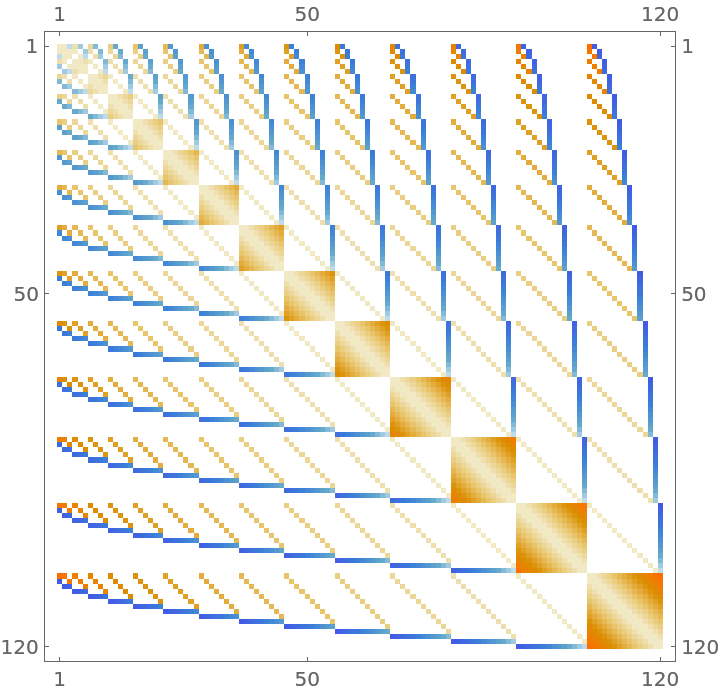
Neat Examples (1)
Visualize the structure of a bialternate sum:


![Clear[x, y, \[Alpha], \[Beta]];
Brusselator[{x_, y_}][{\[Alpha]_, \[Beta]_}] := {\[Alpha] - (\[Beta] + 1) x + x^2 y, \[Beta] x - x^2 y};
X = {x, y};
\[Mu] = {\[Alpha], \[Beta]};
Brusselator[X][\[Mu]] // Column](https://www.wolframcloud.com/obj/resourcesystem/images/c85/c854493c-4e88-4b85-b37e-294c38ed77e6/380439521a405a6a.png)
![Clear[x, y, z, \[Alpha], \[Beta]];
Lure[{x_, y_, z_}][{\[Alpha]_, \[Beta]_}] := {y, z, -x + x^2 - \[Beta] y - \[Alpha] z};
X = {x, y, z};
\[Mu] = {\[Alpha], \[Beta]};
Lure[X][\[Mu]] // Column](https://www.wolframcloud.com/obj/resourcesystem/images/c85/c854493c-4e88-4b85-b37e-294c38ed77e6/52c7c3ec589347e0.png)


![Clear[x, y, z, \[Sigma], r, \[Beta]];
Lorenz[{x_, y_, z_}][{\[Sigma]_, r_, \[Beta]_}] := {\[Sigma] (y - x), -x z + r x - y, x y - \[Beta] z};
X = {x, y, z};
\[Mu] = {\[Sigma], r, \[Beta]};
Lorenz[X][\[Mu]] // Column](https://www.wolframcloud.com/obj/resourcesystem/images/c85/c854493c-4e88-4b85-b37e-294c38ed77e6/758520a3dc5d5042.png)


![n = 7;
ResourceFunction["BialternateSum"][
Transpose[Array[\[FormalA], {n, n}]]] == Transpose[
ResourceFunction["BialternateSum"][
Array[\[FormalA], {n, n}]]] // Simplify](https://www.wolframcloud.com/obj/resourcesystem/images/c85/c854493c-4e88-4b85-b37e-294c38ed77e6/4bf92ae005128783.png)
![n = 7;
ResourceFunction["BialternateSum"][
Array[\[FormalA], {n, n}] + Array[\[FormalB], {n, n}]] == ResourceFunction["BialternateSum"][Array[\[FormalA], {n, n}]] + ResourceFunction["BialternateSum"][
Array[\[FormalB], {n, n}]] // Simplify](https://www.wolframcloud.com/obj/resourcesystem/images/c85/c854493c-4e88-4b85-b37e-294c38ed77e6/1a2adf7b27ac2775.png)
![m = \!\(\*
TagBox[
RowBox[{"(", "", GridBox[{
{"18", "52",
RowBox[{"-", "148"}], "148"},
{
RowBox[{"-", "10"}],
RowBox[{"-", "32"}], "100",
RowBox[{"-", "100"}]},
{
RowBox[{"-", "13"}],
RowBox[{"-", "56"}], "173",
RowBox[{"-", "168"}]},
{
RowBox[{"-", "11"}],
RowBox[{"-", "49"}], "150",
RowBox[{"-", "145"}]}
},
GridBoxAlignment->{"Columns" -> {{Center}}, "Rows" -> {{Baseline}}},
GridBoxSpacings->{"Columns" -> {
Offset[0.27999999999999997`], {
Offset[0.7]},
Offset[0.27999999999999997`]}, "Rows" -> {
Offset[0.2], {
Offset[0.4]},
Offset[0.2]}}], "", ")"}],
Function[BoxForm`e$,
MatrixForm[BoxForm`e$]]]\);
eigs = Eigenvalues[m]](https://www.wolframcloud.com/obj/resourcesystem/images/c85/c854493c-4e88-4b85-b37e-294c38ed77e6/27e5eb709323f6bb.png)

![Clear[x, y, z, \[Sigma], r, \[Beta]];
Lorenz[{x_, y_, z_}][{\[Sigma]_, r_, \[Beta]_}] := {\[Sigma] (y - x), -x z + r x - y, x y - \[Beta] z};
X = {x, y, z};
\[Mu] = {\[Sigma], r, \[Beta]};
Lorenz[X][\[Mu]] // Column](https://www.wolframcloud.com/obj/resourcesystem/images/c85/c854493c-4e88-4b85-b37e-294c38ed77e6/66b18684901e3126.png)


![Reduce[Det[A0[\[Mu]]] < 0 && \[Sigma] > 0 && r > 1 && \[Beta] > 0, r] === Reduce[
Reduce[Thread[
DeleteCases[CoefficientList[polJ0, \[Lambda]], _Integer] > 0]] &&
LiuMinor > 0 && \[Sigma] > 0 && r > 1 && \[Beta] > 0, r]](https://www.wolframcloud.com/obj/resourcesystem/images/c85/c854493c-4e88-4b85-b37e-294c38ed77e6/23ab073560c54925.png)