Hopf bifurcation analysis and first Lyapunov coefficient (3)
Compute the first Lyapunov coefficient for the Brusselator system:
The equilibrium point:
Assume fixed and take as a bifurcation parameter to show that the system exhibits a supercritical Hopf bifurcation at , where .
The Jacobian matrix and its transpose:
Analyse the local stability with the resource function BialternateSum, with β as control parameter:
The critical value of the Hopf bifurcation:
Then, the equilibrium of the Brusselator system is locally asymptotically stable for and locally asymptotically unstable for (appears a stable limit cycle surrounded the unstable equilibrium point). We verify the previous conclusion by the transversality condition:
The non-trivial equilibrium point at :
Shift the non-trivial equilibrium point to the origin:
Verify that indeed the non-trivial equilibrium was shifted to the origin:
The Jacobian matrix in the new state variables:
Using both the linear approximation and its transpose at the origin, with and , we obtain the eigenvalues and :
The critical eigenvectors ,  , ,
, ,  :
:
The normalization
The third-order Taylor approximation for the polynomial system
Linear function:
Bilinear function:
Trilinear function:
Verify that the Taylor series expansion of the Brusselator system is correct:
The first Lyapunov coefficient is given by:
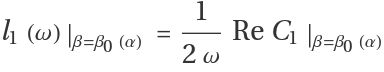
where

and , are given by
,
First, compute , and as follows:
Finally, compute the first Lyapunov coefficient:
The first Lyapunov coefficient is clearly negative for all positive . Thus, the Hopf bifurcation is nondegenerate and always supercritical.
Compute the first Lyapunov coefficient for the following predator-prey system:
The orbitally equivalent polynomial system:
The Jacobian matrix for the orbitally equivalent polynomial system:
The non-trivial equilibrium point:
The linear approximation at :
Analyse the local stability with the resource function BialternateSum, with as control parameter:
The critical value of the Hopf bifurcation:
Then, is locally asymptotically stable for and locally asymptotically unstable for (with ), and can be confirmed by the transversality condition:
The non-trivial equilibrium point at :
Shift the non-trivial equilibrium point to the origin:
Verify that indeed the non-trivial equilibrium was shifted to the origin:
The Jacobian matrix in the new state variables:
Using both the linear approximation and its transpose at the origin, with  and
and  , we obtain the eigenvalues and :
The critical eigenvectors ,  , ,
, ,  :
:
The normalization
The third-order Taylor approximation for the polynomial system
Linear function:
Bilinear function:
Trilinear function:
Verify that the Taylor series expansion of the polynomial system is correct:
The first Lyapunov coefficient is given by:
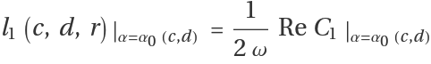
where

and , are given by
,
First, compute , and as follows:
Finally, we compute the first Lyapunov coefficient:
Clearly, the first Lyapunov coefficient is strictly negative for all combinations of the fixed parameters. Therefore, a unique limit cycle emerges from the non-trivial equilibrium via Hopf bifurcation for .
Compute the first Lyapunov coefficient for the following nonlinear feedback-control system of Lur'e type:
For all values of , the Lur'e system has two equilibria, the origin and . At the origin, this system exhibits a supercritical Hopf bifurcation when , where  :
:
The Jacobian matrix and its transpose:
Analyse the local stability with the resource function BialternateSum, with as control parameter:
The critical value of the Hopf bifurcation:
Then, the equilibrium of the Lur'e system is locally asymptotically stable for and locally asymptotically unstable for (appears a stable limit cycle surrounded the unstable equilibrium point). We verify the previous conclusion by the transversality condition:
Using both the linear approximation and its transpose at the origin, with  and , we obtain the eigenvalues and :
The critical eigenvectors ,  , ,
, ,  :
:
The normalization
The third-order Taylor approximation for the polynomial system
Linear function:
Bilinear function:
Trilinear function:
We verify that the Taylor series expansion of the Lur'e system is correct:
The first Lyapunov coefficient is given by:
where

and , are given by
,
First, compute , and
Finally, compute the first Lyapunov coefficient:
The first Lyapunov coefficient is strictly negative for all positive . Thus, the Hopf bifurcation is nondegenerate and always supercritical.
Neimark-Sacker bifurcation analysis and first Lyapunov coefficient (19)
Let's delve into a discrete population model by leveraging the capabilities of the DVectorField function. In this framework, the population at a given time is determined by its value at the previous moment. Specifically, the growth rate of our population is influenced by intraspecific competition, where the current population has a limiting effect on its future growth. Through this approach, interactions can be depicted discretely at each time step, providing a comprehensive view of population dynamics.
Define the previously described discrete-time dynamical system as follows:
Jacobian matrix:
The non-trivial fixed point:
The linear approximation at :
The eigenvalues of the linear approximation :
For the eigenvalues are complex, so the following shift is made in the growth rate to handle this restriction, and then the eigenvalues of are computed again:
The value where the fixed point loses its stability, giving rise to a Neimark-Sacker bifurcation, is given by:
Therefore, the fixed point loses its stability at as verified below:
The linear approximation at the critical bifurcation value and its transpose:
The critical multipliers are given by:
The transversality condition:
The nondegeneracy condition:
for
The critical eigenvectors ,  , ,
, ,  :
:
The normalization
The bilinear and trilinear forms to compute the first Lyapunov coefficient:
The first Lyapunov coefficient (additional nondegeneracy condition) is given by

Finally, compute the first Lyapunov coefficient:
Therefore, a unique and stable closed invariant curve bifurcates from the non-trivial fixed point for .
Quadratic coefficients of the normal form for Bogdanov-Takens bifurcation (15)
Compute the quadratic coefficients of the Bogdanov-Takens bifurcation normal form for a predator-prey model with non-linear predator reproduction and prey competition:
The Jacobian matrix:
Look for the Bogdanov-Takens point:
To explicitly handle constraint  , apply the following shift to get the Bogdanov-Takens point:
With the above shift in the predator population, the equilibrium point of coexistence and the critical value of bifurcation are as follows:
The linear approximation at :
Verify that has a pair of null eigenvalues:
The critical right eigenvectors and :
Verify the conditions and
The transition matrix with the critical right eigenvectors:
The critical left eigenvectors and :
Verify the conditions and
Finally, verify the conditions , and that the matrix is similar to a simple Jordan block:
The quadratic coefficients, involved in the nondegeneracy condition, can be computed in the following two ways:
The Bogdanov-Takens bifurcation in this case is non-degenerate when and the unique point of degeneracy is:


![Lorenz[{x_, y_, z_}][{\[Sigma]_, r_, \[Beta]_}] := {\[Sigma] (y - x), -x z + r x - y, x y - \[Beta] z};
X = {x, y, z};
\[Mu] = {\[Sigma], r, \[Beta]};
Column@Lorenz[X][\[Mu]]](https://www.wolframcloud.com/obj/resourcesystem/images/d71/d71db709-5757-44e8-a522-45a3bdfaf3d6/6dd90e063b212826.png)

![X0[{\[Sigma]_, r_, \[Beta]_}] := Evaluate[SolveValues[Lorenz[X][\[Mu]] == 0, X]]
X1[{\[Sigma]_, r_, \[Beta]_}] = Part[X0[\[Mu]], 1];
X2[{\[Sigma]_, r_, \[Beta]_}] = Part[X0[\[Mu]], 2];
X3[{\[Sigma]_, r_, \[Beta]_}] = Part[X0[\[Mu]], 3];
Column@Map[Composition[MatrixForm, List], List[X1[\[Mu]], X2[\[Mu]], X3[\[Mu]]]]](https://www.wolframcloud.com/obj/resourcesystem/images/d71/d71db709-5757-44e8-a522-45a3bdfaf3d6/5aa2f623dfb1bd92.png)

![Column[Map[
MatrixForm@
ResourceFunction["DVectorField"][Lorenz[X][\[Mu]], X, #, 1, "MultilinearFunction"] &, {X1[\[Mu]], X2[\[Mu]], X3[\[Mu]]}], Spacings -> 1]](https://www.wolframcloud.com/obj/resourcesystem/images/d71/d71db709-5757-44e8-a522-45a3bdfaf3d6/279a06fbedb927d0.png)

![Column[Map[
MatrixForm@
ResourceFunction["DVectorField"][Lorenz[X][\[Mu]], X, #, 2, "MultilinearFunction"] &, {X1[\[Mu]], X2[\[Mu]], X3[\[Mu]]}], Spacings -> 1]](https://www.wolframcloud.com/obj/resourcesystem/images/d71/d71db709-5757-44e8-a522-45a3bdfaf3d6/61ff7d0d695a0f79.png)

![Clear[X, \[Mu]]
Brusselator[{x_, y_}][{\[Alpha]_, \[Beta]_}] := {\[Alpha] - (\[Beta] + 1) x + x^2 y, \[Beta] x - x^2 y}
X = {x, y};
\[Mu] = {\[Alpha], \[Beta]};
Column@Brusselator[X][\[Mu]]](https://www.wolframcloud.com/obj/resourcesystem/images/d71/d71db709-5757-44e8-a522-45a3bdfaf3d6/03a89006473aebb0.png)
![Clear[X0]
X0[{\[Alpha]_, \[Beta]_}] := Evaluate@SolveValues[Brusselator[X][\[Mu]] == 0, X][[1]]
MatrixForm@List@X0[\[Mu]]](https://www.wolframcloud.com/obj/resourcesystem/images/d71/d71db709-5757-44e8-a522-45a3bdfaf3d6/1a9452faec3691ff.png)
![\[Beta]0 = Part[Normal[
SolveValues[
Det[ResourceFunction["BialternateSum"][J[X0[\[Mu]]][\[Mu]]]] == 0 && \[Alpha] > 0 && \[Beta] > 0, \[Beta]]], 1]](https://www.wolframcloud.com/obj/resourcesystem/images/d71/d71db709-5757-44e8-a522-45a3bdfaf3d6/6e95bcd488743fd8.png)
![Brusselator[{\[Xi]_, \[Eta]_}][\[Alpha]_] := Evaluate@
Collect[ReplaceAll[Thread[{x, y} -> {\[Xi], \[Eta]}]][
Brusselator[
X + X0\[Beta]0][{\[Alpha], \[Beta]0}]], {\[Xi], \[Eta]}, FullSimplify]
X = {\[Xi], \[Eta]};
Column@Brusselator[X][\[Alpha]]](https://www.wolframcloud.com/obj/resourcesystem/images/d71/d71db709-5757-44e8-a522-45a3bdfaf3d6/36aa8b3c766d79cb.png)

![Clear[J]
J[{\[Xi]_, \[Eta]_}][\[Alpha]_] := Evaluate[
Collect[D[Brusselator[X][\[Alpha]], {X}], {\[Xi], \[Eta]}, FullSimplify]]
MatrixForm@J[X][\[Alpha]]](https://www.wolframcloud.com/obj/resourcesystem/images/d71/d71db709-5757-44e8-a522-45a3bdfaf3d6/69dd7bc37b429ba9.png)

![origin = {0, 0};
\[Alpha] = \[Omega];
J0[\[Omega]_] := Simplify@J[origin][\[Alpha]]
MatrixForm@J0[\[Omega]]](https://www.wolframcloud.com/obj/resourcesystem/images/d71/d71db709-5757-44e8-a522-45a3bdfaf3d6/40e4978c8cef1780.png)
![q = Eigenvectors[J0[\[Omega]]][[2]];
qc = ComplexExpand[Conjugate[q]];
pc = Eigenvectors[J0T[\[Omega]]][[1]];
p = ComplexExpand[Conjugate[pc]];
Row[Map[Composition[MatrixForm, List], {q, qc, p, pc}], " "]](https://www.wolframcloud.com/obj/resourcesystem/images/d71/d71db709-5757-44e8-a522-45a3bdfaf3d6/7166bd75b397c4ec.png)
![pn = 1/cn p;
Row[Map[Composition[MatrixForm, List, Simplify], {pn, J0T[\[Alpha]] . pn - I \[Omega]*pn}], " "]](https://www.wolframcloud.com/obj/resourcesystem/images/d71/d71db709-5757-44e8-a522-45a3bdfaf3d6/120a26f810cb523f.png)
![Row[Map[Composition[Simplify, MatrixForm, List], {J0[\[Alpha]] . q - I \[Omega]*q, J0[\[Alpha]] . qc + I \[Omega]*qc, J0T[\[Alpha]] . pn - I \[Omega]*pn, J0T[\[Alpha]] . pc + I \[Omega]*pc}], " "]](https://www.wolframcloud.com/obj/resourcesystem/images/d71/d71db709-5757-44e8-a522-45a3bdfaf3d6/37c3b468043b6917.png)
![AA[{\[Xi]1_, \[Eta]1_}][\[Alpha]_] := Evaluate[
ResourceFunction["DVectorField"][Brusselator[X][\[Alpha]], X, origin, 1, "MultilinearFunction"]]
MatrixForm@AA[{\[Xi]1, \[Eta]1}][\[Omega]]](https://www.wolframcloud.com/obj/resourcesystem/images/d71/d71db709-5757-44e8-a522-45a3bdfaf3d6/118314cc066cdf60.png)
![BB[{\[Xi]1_, \[Eta]1_}, {\[Xi]2_, \[Eta]2_}][\[Alpha]_] := Evaluate[
ResourceFunction["DVectorField"][Brusselator[X][\[Alpha]], X, origin, 2, "MultilinearFunction"]]
MatrixForm@BB[{\[Xi]1, \[Eta]1}, {\[Xi]2, \[Eta]2}][\[Omega]]](https://www.wolframcloud.com/obj/resourcesystem/images/d71/d71db709-5757-44e8-a522-45a3bdfaf3d6/36123ba5b9073352.png)

![CC[{\[Xi]1_, \[Eta]1_}, {\[Xi]2_, \[Eta]2_}, {\[Xi]3_, \[Eta]3_}][\[Alpha]_] := Evaluate[
ResourceFunction["DVectorField"][Brusselator[X][\[Alpha]], X, origin, 3, "MultilinearFunction"]]
MatrixForm@
CC[{\[Xi]1, \[Eta]1}, {\[Xi]2, \[Eta]2}, {\[Xi]3, \[Eta]3}][\[Omega]]](https://www.wolframcloud.com/obj/resourcesystem/images/d71/d71db709-5757-44e8-a522-45a3bdfaf3d6/7d0ac10f57df3091.png)
![MatrixForm@{FullSimplify[
Brusselator[X][\[Omega]] - (AA[{\[Xi], \[Eta]}][\[Omega]] + BB[{\[Xi], \[Eta]}, {\[Xi], \[Eta]}][\[Omega]]/2! + CC[{\[Xi], \[Eta]}, {\[Xi], \[Eta]}, {\[Xi], \[Eta]}][\[Omega]]/3!) /. {\[Xi] -> t \[Xi], \[Eta] -> t \[Eta]}]}](https://www.wolframcloud.com/obj/resourcesystem/images/d71/d71db709-5757-44e8-a522-45a3bdfaf3d6/019326ff31b60075.png)
![Clear[X, \[Mu]]
PredatorPrey[{x_, y_}][{c_, d_, r_, \[Alpha]_}] := {r x (1 - x) - (
c x y)/(x + \[Alpha]), -d y + (c x y)/(x + \[Alpha])}
X = {x, y};
\[Mu] = {c, d, r, \[Alpha]};
Column[PredatorPrey[X][\[Mu]]]](https://www.wolframcloud.com/obj/resourcesystem/images/d71/d71db709-5757-44e8-a522-45a3bdfaf3d6/5bc5ffe0756f4008.png)

![PolynomialPredatorPrey[{x_, y_}][{c_, d_, r_, \[Alpha]_}] := Evaluate@
Map[Composition[Total, Factor, MonomialList[#, {x, y}] &, Expand, Factor, Times[#, x + \[Alpha]] &], PredatorPrey[X][\[Mu]]]
Column@PolynomialPredatorPrey[X][\[Mu]]](https://www.wolframcloud.com/obj/resourcesystem/images/d71/d71db709-5757-44e8-a522-45a3bdfaf3d6/305d64c72b033734.png)
![Clear[J]
J[{x_, y_}][{c_, d_, r_, \[Alpha]_}] := Evaluate[Simplify@D[PolynomialPredatorPrey[X][\[Mu]], {X}]]
MatrixForm@J[X][\[Mu]]](https://www.wolframcloud.com/obj/resourcesystem/images/d71/d71db709-5757-44e8-a522-45a3bdfaf3d6/2de2b188cd2b015b.png)
![Clear[X0]
X0[{c_, d_, r_, \[Alpha]_}] := Evaluate[
Simplify[
Normal[SolveValues[
PolynomialPredatorPrey[X][\[Mu]] == 0 && Reduce[Thread[Flatten[{X, \[Mu]}] > 0]], X][[1]]]]]
MatrixForm@List@X0[\[Mu]]](https://www.wolframcloud.com/obj/resourcesystem/images/d71/d71db709-5757-44e8-a522-45a3bdfaf3d6/60e3674b068fb113.png)
![Clear[J0]
J0[{c_, d_, r_, \[Alpha]_}] := Simplify@J[X0[\[Mu]]][\[Mu]]
MatrixForm@J0[\[Mu]]](https://www.wolframcloud.com/obj/resourcesystem/images/d71/d71db709-5757-44e8-a522-45a3bdfaf3d6/52ec819aaa398e3a.png)

![\[Alpha]0 = Part[Normal[
SolveValues[
Det[ResourceFunction["BialternateSum"][J0[\[Mu]]]] == 0 && 0 < d < c && r > 0 && \[Alpha] > 0, \[Alpha]]], 1]](https://www.wolframcloud.com/obj/resourcesystem/images/d71/d71db709-5757-44e8-a522-45a3bdfaf3d6/73585ed9fd702550.png)
![PolynomialPredatorPrey[{\[Xi]_, \[Eta]_}][{c_, d_, r_}] := Evaluate@
Map[Composition[Total, Collect[#, {\[Xi], \[Eta]}, FullSimplify] &, MonomialList[#, {\[Xi], \[Eta]}] &], ReplaceAll[Thread[{x, y} -> {\[Xi], \[Eta]}]][
PolynomialPredatorPrey[X + X0\[Alpha]0][{c, d, r, \[Alpha]0}]]]
X = {\[Xi], \[Eta]};
\[Mu]3 = {c, d, r};
Column[PolynomialPredatorPrey[X][\[Mu]3]]](https://www.wolframcloud.com/obj/resourcesystem/images/d71/d71db709-5757-44e8-a522-45a3bdfaf3d6/7a0f94697b3ad2e1.png)

![J[{\[Xi]_, \[Eta]_}][{c_, d_, r_}] := Evaluate[
Collect[D[PolynomialPredatorPrey[X][\[Mu]3], {X}], {\[Xi], \[Eta]}, FullSimplify]]
MatrixForm@J[X][\[Mu]3]](https://www.wolframcloud.com/obj/resourcesystem/images/d71/d71db709-5757-44e8-a522-45a3bdfaf3d6/49621cfc875cf4a3.png)

![Clear[origin]
origin = {0, 0};
r0 = ((c + d)^3 \[Omega]^2)/(c^2 (c - d) d);
\[Mu]2 = {c, d};](https://www.wolframcloud.com/obj/resourcesystem/images/d71/d71db709-5757-44e8-a522-45a3bdfaf3d6/27c19aa2832d7856.png)
![Clear[J0]
J0[{c_, d_}] := Simplify@J[origin][{c, d, r0}]
MatrixForm@J0[\[Mu]2]](https://www.wolframcloud.com/obj/resourcesystem/images/d71/d71db709-5757-44e8-a522-45a3bdfaf3d6/2f3af6fe2eb016ef.png)

![Clear[J0T]
J0T[{c_, d_}] := Simplify@Transpose[J[origin][{c, d, r0}]]
MatrixForm@J0T[\[Mu]2]](https://www.wolframcloud.com/obj/resourcesystem/images/d71/d71db709-5757-44e8-a522-45a3bdfaf3d6/4ba48d7b23616f1f.png)

![Clear[q, qc, pc, p]
q = -I \[Omega] (c + d)*Eigenvectors[J0[\[Mu]2]][[2]];
qc = ComplexExpand[Conjugate[q]];
pc = -I c d*Eigenvectors[J0T[\[Mu]2]][[1]];
p = ComplexExpand[Conjugate[pc]];
Row[Map[Composition[MatrixForm, List], {q, qc, p, pc}], " "]](https://www.wolframcloud.com/obj/resourcesystem/images/d71/d71db709-5757-44e8-a522-45a3bdfaf3d6/4645fd7c553df120.png)
![Clear[pn]
pn = 1/cn p;
Row[Map[Composition[MatrixForm, List, Simplify], {pn, J0T[\[Mu]2] . pn - I \[Omega]*pn}], " "]](https://www.wolframcloud.com/obj/resourcesystem/images/d71/d71db709-5757-44e8-a522-45a3bdfaf3d6/1dee4a722366e70d.png)
![Row[Map[Composition[MatrixForm, List, Simplify], {J0[\[Mu]2] . q - I \[Omega]*q, J0[\[Mu]2] . qc + I \[Omega]*qc, J0T[\[Mu]2] . pn - I \[Omega]*pn, J0T[\[Mu]2] . pc + I \[Omega]*pc}], " "]](https://www.wolframcloud.com/obj/resourcesystem/images/d71/d71db709-5757-44e8-a522-45a3bdfaf3d6/4b29c31fbc1b486f.png)
![Clear[AA]
AA[{\[Xi]1_, \[Eta]1_}][{c_, d_, r_}] := Evaluate[
ResourceFunction["DVectorField"][PolynomialPredatorPrey[X][\[Mu]3], X, origin, 1, "MultilinearFunction"]]
MatrixForm@AA[{\[Xi]1, \[Eta]1}][\[Mu]3]](https://www.wolframcloud.com/obj/resourcesystem/images/d71/d71db709-5757-44e8-a522-45a3bdfaf3d6/5c850d99be8ba4e0.png)

![Clear[BB]
BB[{\[Xi]1_, \[Eta]1_}, {\[Xi]2_, \[Eta]2_}][{c_, d_, r_}] := Evaluate[
ResourceFunction["DVectorField"][PolynomialPredatorPrey[X][\[Mu]3], X, origin, 2, "MultilinearFunction"]]
MatrixForm@BB[{\[Xi]1, \[Eta]1}, {\[Xi]2, \[Eta]2}][\[Mu]3]](https://www.wolframcloud.com/obj/resourcesystem/images/d71/d71db709-5757-44e8-a522-45a3bdfaf3d6/24c41ab7d2dc3f86.png)

![Clear[CC]
CC[{\[Xi]1_, \[Eta]1_}, {\[Xi]2_, \[Eta]2_}, {\[Xi]3_, \[Eta]3_}][{c_,
d_, r_}] := Evaluate[
ResourceFunction["DVectorField"][PolynomialPredatorPrey[X][\[Mu]3], X, origin, 3, "MultilinearFunction"]]
MatrixForm@
CC[{\[Xi]1, \[Eta]1}, {\[Xi]2, \[Eta]2}, {\[Xi]3, \[Eta]3}][\[Mu]3]](https://www.wolframcloud.com/obj/resourcesystem/images/d71/d71db709-5757-44e8-a522-45a3bdfaf3d6/410841639822a9b4.png)
![MatrixForm@{FullSimplify[
PolynomialPredatorPrey[X][{c, d, r0}] - (AA[{\[Xi], \[Eta]}][{c, d, r0}] + BB[{\[Xi], \[Eta]}, {\[Xi], \[Eta]}][{c, d, r0}]/2! + CC[{\[Xi], \[Eta]}, {\[Xi], \[Eta]}, {\[Xi], \[Eta]}][{c, d, r0}]/3!) /. {\[Xi] -> t \[Xi], \[Eta] -> t \[Eta]}]}](https://www.wolframcloud.com/obj/resourcesystem/images/d71/d71db709-5757-44e8-a522-45a3bdfaf3d6/7a0c004510d19af7.png)
![Clear[h20]
h20 = Simplify[(Inverse[
2 I \[Omega]*IdentityMatrix[2] - J0[\[Mu]2]]) . BB[q, q][\[Mu]3]];
MatrixForm@List@h20](https://www.wolframcloud.com/obj/resourcesystem/images/d71/d71db709-5757-44e8-a522-45a3bdfaf3d6/5954b167c41ac497.png)
![Clear[h11]
h11 = Simplify[-Inverse[J0[\[Mu]2]] . BB[q, qc][\[Mu]3]];
MatrixForm@List@h11](https://www.wolframcloud.com/obj/resourcesystem/images/d71/d71db709-5757-44e8-a522-45a3bdfaf3d6/49079c52eb67442c.png)

![Clear[L1]
L1 = FullSimplify[1/(2 \[Omega]) ComplexExpand[Re[C1]]]](https://www.wolframcloud.com/obj/resourcesystem/images/d71/d71db709-5757-44e8-a522-45a3bdfaf3d6/08a56ede14d65013.png)
![Clear[X, \[Mu]]
Lure[{x_, y_, z_}][{\[Alpha]_, \[Beta]_}] := {y, z, -x + x^2 - \[Beta] y - \[Alpha] z};
X = {x, y, z};
\[Mu] = {\[Alpha], \[Beta]};
Column@Lure[X][\[Mu]]](https://www.wolframcloud.com/obj/resourcesystem/images/d71/d71db709-5757-44e8-a522-45a3bdfaf3d6/34c2b1fe1e23727a.png)

![Clear[X0]
X0[{\[Alpha]_, \[Beta]_}] := Evaluate[SolveValues[Lure[X][\[Mu]] == 0, X]]
Row@Map[Composition[MatrixForm, List], X0[\[Mu]]]](https://www.wolframcloud.com/obj/resourcesystem/images/d71/d71db709-5757-44e8-a522-45a3bdfaf3d6/40c9670db2431df4.png)
![Clear[J]
J[{x_, y_, z_}][{\[Alpha]_, \[Beta]_}] := Evaluate[D[Lure[X][\[Mu]], {X}]]
MatrixForm@J[X][\[Mu]]](https://www.wolframcloud.com/obj/resourcesystem/images/d71/d71db709-5757-44e8-a522-45a3bdfaf3d6/5f888d8c6f7b09b8.png)

![Clear[Jt]
Jt[{x_, y_, z_}][{\[Alpha]_, \[Beta]_}] := Evaluate[Transpose[J[X][\[Mu]]]]
MatrixForm@Jt[X][\[Mu]]](https://www.wolframcloud.com/obj/resourcesystem/images/d71/d71db709-5757-44e8-a522-45a3bdfaf3d6/21195103b28e299c.png)

![Clear[\[Alpha]0]
\[Alpha]0 = Part[Normal[
SolveValues[
Det[ResourceFunction["BialternateSum"][
J[X0[\[Mu]][[1]]][\[Mu]]]] == 0 && \[Alpha] > 0 && \[Beta] > 0, \[Alpha]]], 1]](https://www.wolframcloud.com/obj/resourcesystem/images/d71/d71db709-5757-44e8-a522-45a3bdfaf3d6/7af2f67656d76845.png)
![Clear[J0]
\[Beta] = \[Omega]^2;
J0[\[Omega]_] := Simplify@J[X0[{\[Alpha]0, \[Beta]}][[1]]][{\[Alpha]0, \[Beta]}]
MatrixForm[J0[\[Omega]]]](https://www.wolframcloud.com/obj/resourcesystem/images/d71/d71db709-5757-44e8-a522-45a3bdfaf3d6/481e6d6aae50cbcb.png)

![Clear[J0T]
J0T[\[Omega]_] := Simplify@Transpose[J0[\[Omega]]]
MatrixForm[J0T[\[Omega]]]](https://www.wolframcloud.com/obj/resourcesystem/images/d71/d71db709-5757-44e8-a522-45a3bdfaf3d6/4a0520854a729347.png)


![Clear[q, qc, p, pc]
q = -\[Omega]^2*Eigenvectors[J0[\[Omega]]][[3]];
qc = ComplexExpand[Conjugate[q]];
p = -\[Omega]^2*Eigenvectors[J0T[\[Omega]]][[2]] // Expand;
pc = ComplexExpand[Conjugate[p]];
Row[Map[Composition[MatrixForm, List], {q, qc, p, pc}], " "]](https://www.wolframcloud.com/obj/resourcesystem/images/d71/d71db709-5757-44e8-a522-45a3bdfaf3d6/5060d130fc327ab4.png)
![Clear[pn]
pn = Map[Total, MapAt[Composition[FullSimplify, Times[#, I] &], ComplexExpand@ReIm[1/cn pc], {All, 2}]];
Row[Map[Composition[MatrixForm, List, Simplify], {pn, J0T[\[Omega]] . pn - I \[Omega]*pn}], " "]](https://www.wolframcloud.com/obj/resourcesystem/images/d71/d71db709-5757-44e8-a522-45a3bdfaf3d6/1ad6b2b30fa457e2.png)
![Row[Map[Composition[Simplify, MatrixForm, List], {J0[\[Alpha]] . q - I \[Omega]*q, J0[\[Alpha]] . qc + I \[Omega]*qc, J0T[\[Alpha]] . p + I \[Omega]*p, J0T[\[Alpha]] . pn - I \[Omega]*pn}], " "]](https://www.wolframcloud.com/obj/resourcesystem/images/d71/d71db709-5757-44e8-a522-45a3bdfaf3d6/542fe224340670ba.png)
![Clear[AA]
AA[{x1_, y1_, z1_}][\[Omega]_] := Evaluate[
ResourceFunction["DVectorField"][Lure[X][{\[Alpha]0, \[Beta]}], X, X0[{\[Alpha]0, \[Beta]}][[1]], 1, "MultilinearFunction"]]
MatrixForm@AA[{x1, y1, z1}][\[Omega]]](https://www.wolframcloud.com/obj/resourcesystem/images/d71/d71db709-5757-44e8-a522-45a3bdfaf3d6/60e532d16951d47c.png)

![Clear[BB]
BB[{x1_, y1_, \[FormalZ]1_}, {x2_, y2_, z2_}][\[Omega]_] := Evaluate[
ResourceFunction["DVectorField"][Lure[X][{\[Alpha]0, \[Beta]}], X, X0[{\[Alpha]0, \[Beta]}][[1]], 2, "MultilinearFunction"]]
MatrixForm@BB[{x1, y1, z1}, {x2, y2, z2}][\[Omega]]](https://www.wolframcloud.com/obj/resourcesystem/images/d71/d71db709-5757-44e8-a522-45a3bdfaf3d6/622bcca1e97cadfa.png)
![Clear[CC]
CC[{x1_, y1_, z1_}, {x2_, y2_, z2_}, {x3_, y3_, z3_}][\[Omega]_] := Evaluate[
ResourceFunction["DVectorField"][Lure[X][{\[Alpha]0, \[Beta]}], X, X0[{\[Alpha]0, \[Beta]}][[1]], 3, "MultilinearFunction"]]
MatrixForm@CC[{x1, y1, z1}, {x2, y2, z2}, {x3, y3, z3}][\[Omega]]](https://www.wolframcloud.com/obj/resourcesystem/images/d71/d71db709-5757-44e8-a522-45a3bdfaf3d6/7b8de9967c48f3db.png)
![MatrixForm@{FullSimplify[
Lure[X][{\[Alpha]0, \[Beta]}] - (AA[X][\[Omega]] + BB[X, X][\[Omega]]/2! + CC[X, X, X][\[Omega]]/3!) /. {x -> t x,
y -> t y, z -> t z}]}](https://www.wolframcloud.com/obj/resourcesystem/images/d71/d71db709-5757-44e8-a522-45a3bdfaf3d6/140cc898c0a90471.png)
![Clear[h20]
h20 = (Inverse[2 I \[Omega]*IdentityMatrix[3] - J0[\[Omega]]]) . BB[q, q][\[Omega]];
MatrixForm[{h20}]](https://www.wolframcloud.com/obj/resourcesystem/images/d71/d71db709-5757-44e8-a522-45a3bdfaf3d6/050c433580d51e96.png)
![Clear[h11]
h11 = -Inverse[J0[\[Omega]]] . BB[q, qc][\[Omega]];
MatrixForm[{h11}]](https://www.wolframcloud.com/obj/resourcesystem/images/d71/d71db709-5757-44e8-a522-45a3bdfaf3d6/27cc6181e35b64dc.png)
![Clear[L1]
L1 = Factor[
1/(2 \[Omega]) ComplexExpand[Re[C1]] /. \[Omega] -> \[Omega]0];
{num, den} = L1 /. a_/b_ :> {Numerator[a/b], Denominator[a/b]};
numRule = Simplify@(Times @@ Most@#*Last@# &@FactorList[num][[All, 1]]);
denRule = Simplify@*Times @@ Most@#*Last@# &@FactorList[den][[All, 1]];
#[[1]]/#[[2]] &@ReplacePart[{num, den}, {1 -> numRule, 2 -> denRule}]](https://www.wolframcloud.com/obj/resourcesystem/images/d71/d71db709-5757-44e8-a522-45a3bdfaf3d6/67d41fd252c8e407.png)
![Clear[X]
LogisticMap[{x_, y_}][r_] := {r x (1 - y), x}
X = {x, y};
Column@LogisticMap[X][r]](https://www.wolframcloud.com/obj/resourcesystem/images/d71/d71db709-5757-44e8-a522-45a3bdfaf3d6/286c42a72a53b1a0.png)
![Clear[J]
J[{x_, y_}][r_] := Evaluate[Simplify@D[LogisticMap[X][r], {X}]]
MatrixForm@J[X][r]](https://www.wolframcloud.com/obj/resourcesystem/images/d71/d71db709-5757-44e8-a522-45a3bdfaf3d6/71e232b0df7149a1.png)
![Clear[X0]
X0[r_] := Normal@SolveValues[
LogisticMap[X][r] - X == 0 && r > 0 && x > 0 && y > 0, X][[1]]
MatrixForm@List@X0[r]](https://www.wolframcloud.com/obj/resourcesystem/images/d71/d71db709-5757-44e8-a522-45a3bdfaf3d6/7b2333abe8f3557a.png)
![\[Zeta]1 = E^(I \[Theta]0);
\[Zeta]2 = E^(-I \[Theta]0);
\[Theta]0 = ArcTan[Sqrt[3]];
MatrixForm@List@ComplexExpand@Eigenvalues[A0]](https://www.wolframcloud.com/obj/resourcesystem/images/d71/d71db709-5757-44e8-a522-45a3bdfaf3d6/68747cd0f02a301a.png)
![Clear[q, qc, p, pc]
q = ComplexExpand@Eigenvectors[A0][[1]];
qc = ComplexExpand@Eigenvectors[A0][[2]];
p = ComplexExpand@Eigenvectors[A0T][[1]];
pc = ComplexExpand@Eigenvectors[A0T][[2]];
Row[Map[Composition[MatrixForm, List], {q, qc, p, pc}], " "]](https://www.wolframcloud.com/obj/resourcesystem/images/d71/d71db709-5757-44e8-a522-45a3bdfaf3d6/46c6fa1ffa36d187.png)
![Clear[pn]
pn = ComplexExpand[1/cn p];
MatrixForm@List@pn](https://www.wolframcloud.com/obj/resourcesystem/images/d71/d71db709-5757-44e8-a522-45a3bdfaf3d6/770e1f771a3463ee.png)
![Row[Map[Composition[MatrixForm, List, Simplify], {A0 . q - \[Zeta]1*q,
A0 . qc - \[Zeta]2*qc, A0T . pn - \[Zeta]1*pn, A0T . pc - \[Zeta]2*pc}], " "]](https://www.wolframcloud.com/obj/resourcesystem/images/d71/d71db709-5757-44e8-a522-45a3bdfaf3d6/4b5ebf24439f8417.png)
![Clear[BB]
BB[{x1_, y1_}, {x2_, y2_}][r_] := Evaluate[
ResourceFunction["DVectorField"][LogisticMap[X][r], X, X0[r], 2, "MultilinearFunction"]]
MatrixForm@BB[{x1, y1}, {x2, y2}][r]](https://www.wolframcloud.com/obj/resourcesystem/images/d71/d71db709-5757-44e8-a522-45a3bdfaf3d6/24a7b3dfaf20809c.png)
![Clear[CC]
CC[{x1_, y1_}, {x2_, y2_}, {x3_, y3_}][r_] := Evaluate[
ResourceFunction["DVectorField"][LogisticMap[X][r], X, X0[r], 3, "MultilinearFunction"]]
MatrixForm@CC[{x1, y1}, {x2, y2}, {x3, y3}][r]](https://www.wolframcloud.com/obj/resourcesystem/images/d71/d71db709-5757-44e8-a522-45a3bdfaf3d6/28e588ec06aa0baf.png)
![Clear[PredatorPrey, X, \[Mu]]
PredatorPrey[{x_, y_}][{\[Gamma]_, \[Epsilon]_, n_}] := Evaluate@{x (1 - y) - \[Epsilon] x^2, -\[Gamma] y + (y/(n + y)) x y}
X = {x, y};
\[Mu] = {\[Gamma], \[Epsilon], n};
Column[PredatorPrey[X][\[Mu]]]](https://www.wolframcloud.com/obj/resourcesystem/images/d71/d71db709-5757-44e8-a522-45a3bdfaf3d6/05a2fb89c4bd3896.png)
![Clear[J]
J[{x_, y_}][{\[Gamma]_, \[Epsilon]_, n_}] := Evaluate[Simplify[D[PredatorPrey[X][\[Mu]], {X}]]]
MatrixForm@J[X][\[Mu]]](https://www.wolframcloud.com/obj/resourcesystem/images/d71/d71db709-5757-44e8-a522-45a3bdfaf3d6/25dd0b7ac97e45c6.png)

![BTPoint = First@Factor@(SolveValues[
PredatorPrey[X][\[Mu]] == 0 && Tr[J[X][\[Mu]]] == 0 && Det[J[X][\[Mu]]] == 0, {x, \[Gamma], \[Epsilon], n}] /. y -> \[Zeta]0/(2 (1 + \[Zeta]0)))](https://www.wolframcloud.com/obj/resourcesystem/images/d71/d71db709-5757-44e8-a522-45a3bdfaf3d6/704aa6edef8be63a.png)
![Clear[X0]
X0[\[Zeta]0_] := Evaluate[{BTPoint[[1]], \[Zeta]0/(2 (1 + \[Zeta]0))}]
MatrixForm@List@X0[\[Zeta]0]](https://www.wolframcloud.com/obj/resourcesystem/images/d71/d71db709-5757-44e8-a522-45a3bdfaf3d6/298ff5dee5daf323.png)
![Clear[J0]
J0[\[Zeta]0_] := Simplify@(J[X0[\[Zeta]0]][\[Mu]0[\[Zeta]0]])
MatrixForm@J0[\[Zeta]0]](https://www.wolframcloud.com/obj/resourcesystem/images/d71/d71db709-5757-44e8-a522-45a3bdfaf3d6/5747ef7468e9ae3e.png)


![Clear[BB]
BB[{x1_, y1_}, {x2_, y2_}][\[Zeta]0_] := Evaluate[
ResourceFunction["DVectorField"][PredatorPrey[X][\[Mu]0[\[Zeta]0]], X, X0[\[Zeta]0], 2, "MultilinearFunction"]]
MatrixForm@BB[{x1, y1}, {x2, y2}][\[Zeta]0]](https://www.wolframcloud.com/obj/resourcesystem/images/d71/d71db709-5757-44e8-a522-45a3bdfaf3d6/26df8636208ef603.png)

![Clear[a, b]
D20[\[Zeta]0_] := Evaluate[
Simplify[
ResourceFunction["DVectorField"][PredatorPrey[X][\[Mu]0[\[Zeta]0]],
X, X0[\[Zeta]0], 2]]]
MatrixForm@D20[\[Zeta]0]](https://www.wolframcloud.com/obj/resourcesystem/images/d71/d71db709-5757-44e8-a522-45a3bdfaf3d6/4d5c8bc14e9cd913.png)

![MatrixForm@
ResourceFunction[
"DVectorField"][{-x y^2 z + \[Alpha] - \[Beta] x, -y w + x y^2, x y z + w^2, x y z^2 w^3}, {x, y, z, w}, {1, 1, 0, 1}, 3, "MultilinearFunction"]](https://www.wolframcloud.com/obj/resourcesystem/images/d71/d71db709-5757-44e8-a522-45a3bdfaf3d6/6df71cb26739c98b.png)


![{x1, x2, x3} = Range[3];
MatrixForm@
ResourceFunction[
"DVectorField"][{\[Alpha] - x y^2 + \[Beta] - \[Alpha] x \[Beta], (-y + x y^2) (\[Alpha] + \[Beta])}, {x, y}, {1, 2}, 3, "MultilinearFunction"]](https://www.wolframcloud.com/obj/resourcesystem/images/d71/d71db709-5757-44e8-a522-45a3bdfaf3d6/00cb9dca101ece51.png)
![Clear[x1, x2, x3]
MatrixForm@
ResourceFunction[
"DVectorField"][{\[Alpha] - x y^2 + \[Beta] - \[Alpha] x \[Beta], (-y + x y^2) (\[Alpha] + \[Beta])}, {x, y}, {1, 2}, 3, "MultilinearFunction"]](https://www.wolframcloud.com/obj/resourcesystem/images/d71/d71db709-5757-44e8-a522-45a3bdfaf3d6/465152e6ae47e8b2.png)
![Clear[D20]
D20[{{x1_, y1_}, {x2_, y2_}}] = ResourceFunction["DVectorField"][{x - y^2, 2 y/x}, {x, y}, {1, 2}, 2,
"MultilinearFunction"]](https://www.wolframcloud.com/obj/resourcesystem/images/d71/d71db709-5757-44e8-a522-45a3bdfaf3d6/377b1f6ef6b63f04.png)