Wolfram Language
Paclet Repository
Community-contributed installable additions to the Wolfram Language
Primary Navigation
Categories
Cloud & Deployment
Core Language & Structure
Data Manipulation & Analysis
Engineering Data & Computation
External Interfaces & Connections
Financial Data & Computation
Geographic Data & Computation
Geometry
Graphs & Networks
Higher Mathematical Computation
Images
Knowledge Representation & Natural Language
Machine Learning
Notebook Documents & Presentation
Scientific and Medical Data & Computation
Social, Cultural & Linguistic Data
Strings & Text
Symbolic & Numeric Computation
System Operation & Setup
Time-Related Computation
User Interface Construction
Visualization & Graphics
Random Paclet
Alphabetical List
Using Paclets
Create a Paclet
Get Started
Download Definition Notebook
Learn More about
Wolfram Language
CreateCoil
Guides
Creating Coils
Tech Notes
Physics of Creating Simple, Discrete Coils
Symbols
DesToErr
EllipseCoilPlot3D
EllipseCoilPlot
EllipseFieldPlot2D
EllipseFieldPlot
FindEllipseCoil
FindLoopCoil
FindSaddleCoilAxial
FindSaddleCoilAzimuthal
FindSaddleCoil
HarmonicFieldPlot
LoopCoilPlot3D
LoopCoilPlot
LoopFieldPlot2D
LoopFieldPlot
SaddleCoilPlot3D
SaddleCoilPlot
SaddleFieldPlot2D
SaddleFieldPlot
NoahH`CreateCoil`
L
o
o
p
F
i
e
l
d
P
l
o
t
L
o
o
p
F
i
e
l
d
P
l
o
t
[
{
χ
c
1
,
χ
c
2
,
…
}
,
{
i
χ
1
,
i
χ
2
,
…
}
,
ρ
c
,
n
]
p
l
o
t
s
t
h
e
B
x
,
B
y
a
n
d
B
z
f
i
e
l
d
c
o
m
p
o
n
e
n
t
s
a
l
o
n
g
e
a
c
h
o
f
t
h
e
x
-
,
y
-
a
n
d
z
-
c
o
i
l
a
x
e
s
,
g
e
n
e
r
a
t
e
d
b
y
t
h
e
l
o
o
p
-
b
a
s
e
d
c
o
i
l
w
i
t
h
a
x
i
a
l
s
e
p
a
r
a
t
i
o
n
s
χ
c
1
,
χ
c
2
,
…
,
t
u
r
n
r
a
t
i
o
s
i
χ
1
,
i
χ
2
,
…
,
r
a
d
i
u
s
ρ
c
a
n
d
t
a
r
g
e
t
f
i
e
l
d
h
a
r
m
o
n
i
c
o
f
o
r
d
e
r
n
.
L
o
o
p
F
i
e
l
d
P
l
o
t
[
{
C
o
i
l
χ
c
[
1
]
χ
c
1
,
C
o
i
l
χ
c
[
2
]
χ
c
2
,
…
}
,
…
]
i
s
a
n
a
l
t
e
r
n
a
t
i
v
e
w
a
y
o
f
s
p
e
c
i
f
y
i
n
g
t
h
e
a
x
i
a
l
s
e
p
a
r
a
t
i
o
n
s
χ
c
1
,
χ
c
2
,
…
.
D
e
t
a
i
l
s
a
n
d
O
p
t
i
o
n
s
Examples
(
7
)
Basic Examples
(
4
)
P
l
o
t
t
h
e
B
x
,
B
y
a
n
d
B
z
f
i
e
l
d
c
o
m
p
o
n
e
n
t
s
a
l
o
n
g
e
a
c
h
o
f
t
h
e
x
-
,
y
-
a
n
d
z
-
c
o
i
l
a
x
e
s
,
g
e
n
e
r
a
t
e
d
b
y
t
h
e
l
o
o
p
-
b
a
s
e
d
c
o
i
l
o
p
t
i
m
i
s
e
d
f
o
r
t
h
e
n
=
1
f
i
e
l
d
h
a
r
m
o
n
i
c
,
a
n
d
w
i
t
h
a
r
a
d
i
u
s
o
f
0
.
1
m
e
t
r
e
s
:
I
n
[
1
]
:
=
L
o
o
p
F
i
e
l
d
P
l
o
t
[
{
0
.
3
6
2
,
0
.
5
4
9
,
0
.
6
9
7
}
,
{
1
,
-
2
,
2
}
,
0
.
1
,
1
]
O
u
t
[
1
]
=
Directly use the output of
F
i
n
d
L
o
o
p
C
o
i
l
:
I
n
[
1
]
:
=
s
o
l
s
=
F
i
n
d
L
o
o
p
C
o
i
l
{
1
,
-
2
,
2
}
,
2
,
0
.
1
,
3
2
,
"
C
o
i
l
s
R
e
t
u
r
n
e
d
"
3
O
u
t
[
1
]
=
{
{
C
o
i
l
χ
c
[
1
]
0
.
5
5
4
3
7
2
,
C
o
i
l
χ
c
[
2
]
0
.
6
7
4
7
6
6
,
C
o
i
l
χ
c
[
3
]
0
.
8
6
6
0
2
5
,
D
e
s
T
o
E
r
r
3
4
.
5
1
9
8
}
,
{
C
o
i
l
χ
c
[
1
]
0
.
5
5
3
1
,
C
o
i
l
χ
c
[
2
]
0
.
6
7
3
6
0
8
,
C
o
i
l
χ
c
[
3
]
0
.
8
6
5
1
4
2
,
D
e
s
T
o
E
r
r
3
3
.
5
8
5
2
}
,
{
C
o
i
l
χ
c
[
1
]
0
.
5
5
2
5
9
9
,
C
o
i
l
χ
c
[
2
]
0
.
6
7
3
0
6
5
,
C
o
i
l
χ
c
[
3
]
0
.
8
6
4
6
2
9
,
D
e
s
T
o
E
r
r
3
3
.
2
2
7
7
}
}
I
n
[
2
]
:
=
L
o
o
p
F
i
e
l
d
P
l
o
t
[
F
i
r
s
t
[
s
o
l
s
]
,
{
1
,
-
2
,
2
}
,
0
.
1
,
2
,
I
m
a
g
e
S
i
z
e
S
m
a
l
l
]
O
u
t
[
2
]
=
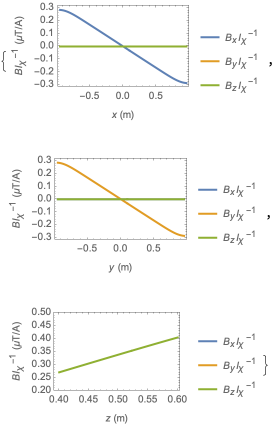
U
s
e
a
u
t
o
m
a
t
i
c
p
l
o
t
r
a
n
g
e
f
o
r
t
h
e
B
-
1
I
χ
v
s
x
a
n
d
B
-
1
I
χ
v
s
y
p
l
o
t
s
,
a
n
d
a
c
u
s
t
o
m
r
a
n
g
e
f
o
r
t
h
e
B
-
1
I
χ
v
s
z
p
l
o
t
(
s
e
e
t
h
e
O
p
t
i
o
n
s
›
P
l
o
t
R
a
n
g
e
s
e
c
t
i
o
n
f
o
r
m
o
r
e
d
e
t
a
i
l
s
o
n
P
l
o
t
R
a
n
g
e
)
:
I
n
[
1
]
:
=
L
o
o
p
F
i
e
l
d
P
l
o
t
[
{
0
.
5
5
,
0
.
6
7
,
0
.
8
7
}
,
{
1
,
-
2
,
2
}
,
1
,
2
,
I
m
a
g
e
S
i
z
e
S
m
a
l
l
,
P
l
o
t
R
a
n
g
e
{
A
u
t
o
m
a
t
i
c
,
A
u
t
o
m
a
t
i
c
,
{
{
0
.
4
,
0
.
6
}
,
{
0
.
2
,
0
.
5
}
}
}
]
O
u
t
[
1
]
=
Open the sections below for more options and examples:
O
p
t
i
o
n
s
(
3
)
S
e
e
A
l
s
o
F
i
n
d
L
o
o
p
C
o
i
l
▪
L
o
o
p
C
o
i
l
P
l
o
t
▪
L
o
o
p
F
i
e
l
d
P
l
o
t
2
D
▪
H
a
r
m
o
n
i
c
F
i
e
l
d
P
l
o
t
▪
S
a
d
d
l
e
F
i
e
l
d
P
l
o
t
▪
E
l
l
i
p
s
e
F
i
e
l
d
P
l
o
t
T
e
c
h
N
o
t
e
s
▪
P
h
y
s
i
c
s
o
f
C
r
e
a
t
i
n
g
S
i
m
p
l
e
,
D
i
s
c
r
e
t
e
C
o
i
l
s
R
e
l
a
t
e
d
G
u
i
d
e
s
▪
C
r
e
a
t
i
n
g
C
o
i
l
s
"
"