Wolfram Function Repository
Instant-use add-on functions for the Wolfram Language
Function Repository Resource:
Interpolate data using polyharmonic splines
ResourceFunction["PolyharmonicSplineInterpolation"][{f1,f2,…}] constructs a polyharmonic spline interpolation of the function values fi, assumed to correspond to x values 1, 2, …. | |
ResourceFunction["PolyharmonicSplineInterpolation"][{{x1,f1},{x2,f2},…}] constructs a polyharmonic spline interpolation of the function values fi corresponding to x values xi. | |
ResourceFunction["PolyharmonicSplineInterpolation"][{{{x1,y1,…},f1},{{x2,y2,…},f2},…}] constructs a polyharmonic spline interpolation of multidimensional data. |
Construct an approximate function that interpolates the data:
| In[1]:= |
Apply the function to find interpolated values:
| In[2]:= |
| Out[2]= |
Plot the interpolation function:
| In[3]:= |
| Out[3]= | 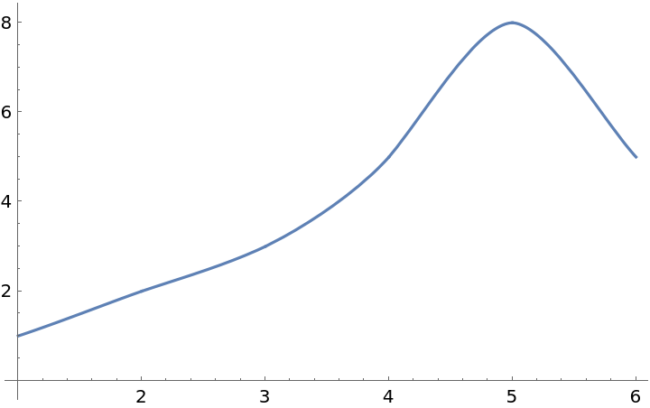 |
Compare with the original data:
| In[4]:= |
| Out[4]= | 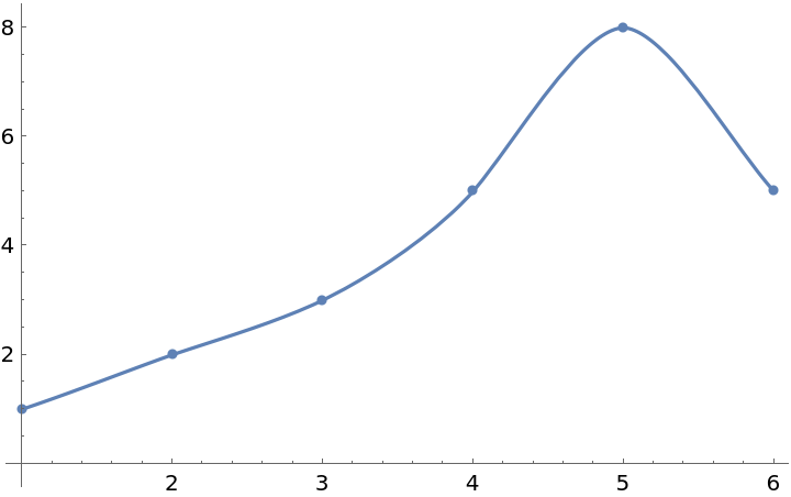 |
Interpolate between points at arbitrary x-values:
| In[5]:= | ![f = ResourceFunction[
"PolyharmonicSplineInterpolation"][{{1., 4.2}, {2., 9.3}, {4., 7.1}, {5., 4.3}, {8., 5.7}, {9., 10.2}, {10., 10.6}, {12., 7.2}}];
Plot[f[x], {x, 1, 12}]](https://www.wolframcloud.com/obj/resourcesystem/images/e86/e86a568f-bbed-4ace-a936-fd225dcb94fe/20a203e64291461f.png) |
| Out[5]= | 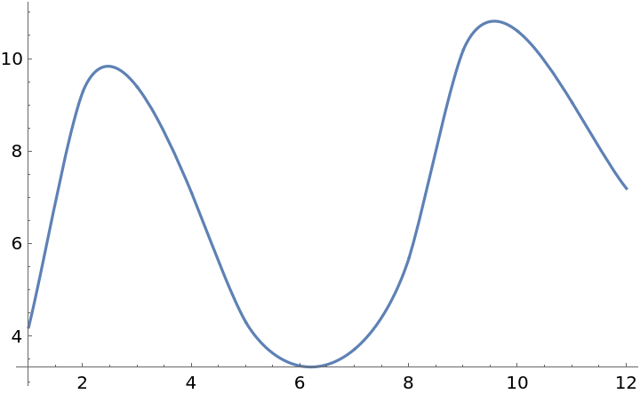 |
Create a list of multidimensional data:
| In[6]:= |
| Out[6]= |
Create a compiled interpolating function:
| In[7]:= |
Plot the interpolating function:
| In[8]:= |
| Out[8]= | 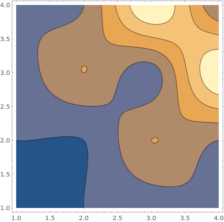 |
Interpolate complex values:
| In[9]:= |
Plot it:
| In[10]:= |
| Out[10]= | 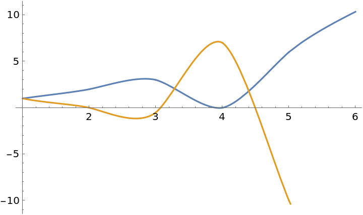 |
Create a list of scattered data:
| In[11]:= |  |
Create a compiled interpolating function:
| In[12]:= |
Plot the interpolating function:
| In[13]:= |
| Out[13]= | 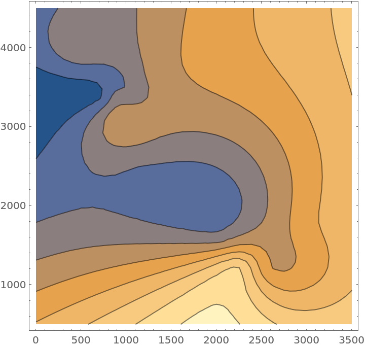 |
Create a vector-valued function of one variable from vector-valued data:
| In[14]:= |
The value is a vector:
| In[15]:= |
| Out[15]= |
Plot both components:
| In[16]:= |
| Out[16]= | 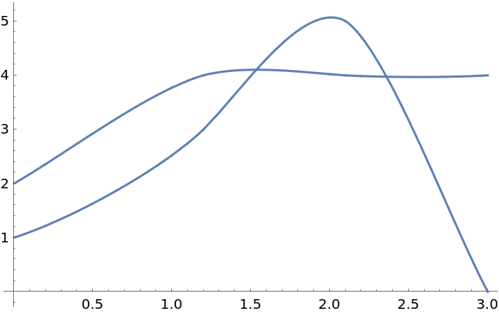 |
Create a vector-valued function of two variables from vector-valued data:
| In[17]:= |
The value is a vector:
| In[18]:= |
| Out[18]= |
Plot3D will show all three components:
| In[19]:= |
| Out[19]= | 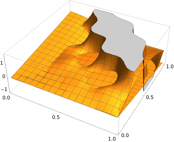 |
A single component may be plotted using Indexed:
| In[20]:= |
| Out[20]= | 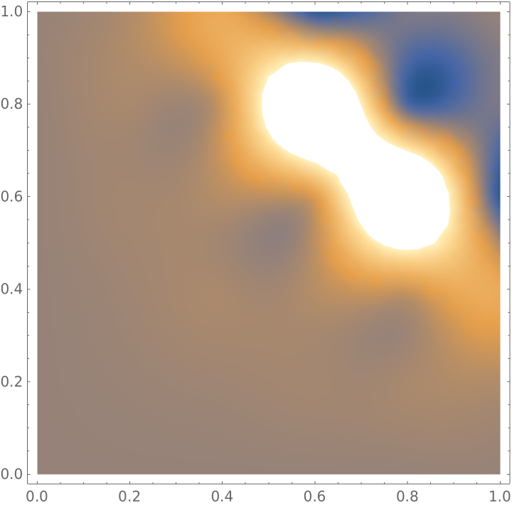 |
Use Compiled→True to generate a compiled function from machine precision data:
| In[21]:= |
| Out[21]= |
A compiled function evaluates more quickly than an uncompiled one:
| In[22]:= |
| Out[22]= |
| In[23]:= |
| Out[23]= |
Compiled→False is appropriate for data with arbitrary precision:
| In[24]:= | ![f = ResourceFunction["PolyharmonicSplineInterpolation"][
N[{{0, 0}, {1/10, 3/10}, {1/2, 3/5}, {1, -1/5}, {2, 3}}, 25], Compiled -> False];
f[3/2]](https://www.wolframcloud.com/obj/resourcesystem/images/e86/e86a568f-bbed-4ace-a936-fd225dcb94fe/0e443f97a1a3aaf6.png) |
| Out[24]= |
Compare interpolating functions of different orders:
| In[25]:= | ![(* Evaluate this cell to get the example input *) CloudGet["https://www.wolframcloud.com/obj/6e1ca173-f435-40bf-9934-36b33666b234"]](https://www.wolframcloud.com/obj/resourcesystem/images/e86/e86a568f-bbed-4ace-a936-fd225dcb94fe/1e94b76b6d337750.png) |
| Out[25]= | 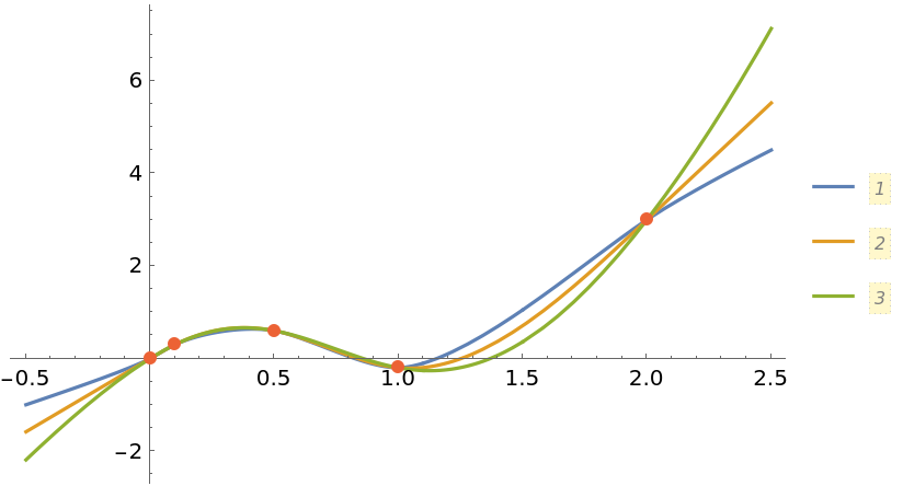 |
The interpolating function always goes through the data points:
| In[26]:= | ![data = {1, 2, 3, 5, 8, 5};
f = ResourceFunction["PolyharmonicSplineInterpolation"][data];
Show[ListPlot[data], Plot[f[x], {x, 1, 6}]]](https://www.wolframcloud.com/obj/resourcesystem/images/e86/e86a568f-bbed-4ace-a936-fd225dcb94fe/5d7c6dc6dbfad118.png) |
| Out[26]= | 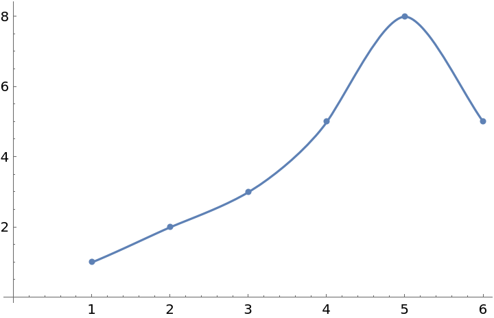 |
This work is licensed under a Creative Commons Attribution 4.0 International License