Details
ResourceFunction["CubicSplineInterpolation"] returns an
InterpolatingFunction object, which can be used like any other pure function.
The interpolation function returned by ResourceFunction["CubicSplineInterpolation"][data] is set up so as to agree with data at every point explicitly specified in data.
ResourceFunction["CubicSplineInterpolation"] yields an interpolant with continuous first and second derivatives.
The function values fi are expected to be real or complex numbers.
The function arguments xi must be real numbers.
ResourceFunction["CubicSplineInterpolation"][data] generates an
InterpolatingFunction object that returns values with the same precision as those in
data.
The following endpoint conditions can be specified for cond:
| "NotAKnot" | not-a-knot end condition |
| "Natural" | natural end condition (zero second derivative) |
| "Clamped" | set derivative at endpoint equal to the derivative of the polynomial passing through first (or last) four points |
| {"Clamped",d} | set derivative at endpoint equal to d |
| {"Clamped",InterpolationOrder→m} | set derivative at endpoint equal to the derivative of the polynomial passing through first (or last) m+1 points |
| "Second" | set second derivative at endpoint equal to 0 |
| {"Second",d} | set second derivative at endpoint equal to d |
| {"Second",InterpolationOrder→m} | set second derivative at endpoint equal to the second derivative of the polynomial passing through first (or last) m+1 points |
| "Periodic" | periodic |
ResourceFunction["CubicSplineInterpolation"][data] is equivalent to ResourceFunction["CubicSplineInterpolation"][data,"Periodic"] if the left and right endpoints of data have the same ordinate, and ResourceFunction["CubicSplineInterpolation"][data,"NotAKnot"] otherwise.
ResourceFunction["CubicSplineInterpolation"][data,{cond1,cond2}] uses cond1 for the left endpoint condition and cond2 for the right endpoint condition.
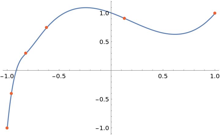
![data = {{-1., -1.}, {-0.96, -0.4}, {-0.82, 0.3}, {-0.62, 0.75}, {0.13,
0.91}, {1., 1.}};
fun = ResourceFunction["CubicSplineInterpolation"][data];
Plot[fun[x], {x, -1, 1}, Epilog -> {Directive[AbsolutePointSize[5], ColorData[97, 4]], Point[data]}, PlotRange -> All]](https://www.wolframcloud.com/obj/resourcesystem/images/481/4810d2d8-5392-4402-8a12-f378111551f4/6c2f8769a39c2d1d.png)
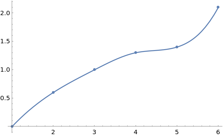
![data = {{0., 0.}, {0.1, 0.3}, {0.5, 0.6}, {1., -0.2}, {2., 3.}};
fun = ResourceFunction["CubicSplineInterpolation"][data, "Natural"];
Plot[fun[x], {x, 0, 2}, Epilog -> {Directive[AbsolutePointSize[5], ColorData[97, 4]], Point[data]}, PlotRange -> All]](https://www.wolframcloud.com/obj/resourcesystem/images/481/4810d2d8-5392-4402-8a12-f378111551f4/6c5d924f76fa7dc1.png)
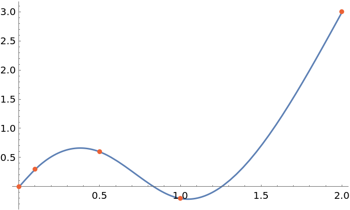
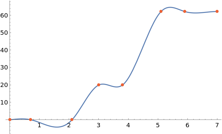
![data = {{0., 0.}, {0.7, 0.02}, {2.1, 0.06}, {3., 20.}, {3.8, 20.}, {5.1, 62.2}, {5.9, 62.24}, {7., 62.26}};
fun = ResourceFunction["CubicSplineInterpolation"][
data, {{"Second", 0.1}, {"Clamped", InterpolationOrder -> 2}}];
Plot[fun[x], {x, 0, 7}, Epilog -> {Directive[AbsolutePointSize[5], ColorData[97, 4]], Point[data]}]](https://www.wolframcloud.com/obj/resourcesystem/images/481/4810d2d8-5392-4402-8a12-f378111551f4/339548e5cc8ea807.png)
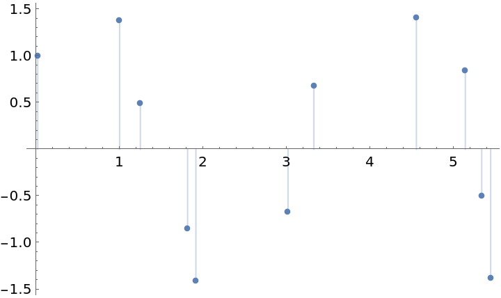
![ts = TemporalData[
TimeSeries, {{{1, Cos[1] + Sin[1], Cos[2] + Sin[2], Cos[3] + Sin[3],
Cos[4] + Sin[4], Cos[5] + Sin[5], Cos[6] + Sin[6], Cos[7] + Sin[7], Cos[8] + Sin[8], Cos[9] + Sin[9], Cos[10] + Sin[10]}}, {{{0.016965744360214943`, 0.9973865299845299, 1.24591736467102, 1.8114088692820352`, 1.9107450982712126`, 3.013995043949912, 3.323754146542503, 4.551557869716615, 5.13709169763333, 5.334143602077121, 5.441221219515277}}}, 1, {"Continuous", 1}, {"Discrete", 1}, 1, {ResamplingMethod -> {"Interpolation", InterpolationOrder -> 1}}},
False, 10.1];
ListPlot[ts, Filling -> Axis]](https://www.wolframcloud.com/obj/resourcesystem/images/481/4810d2d8-5392-4402-8a12-f378111551f4/76c7923042f94d2a.png)
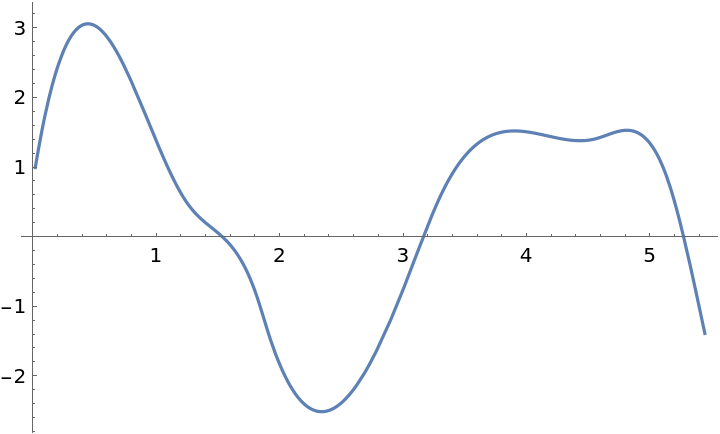
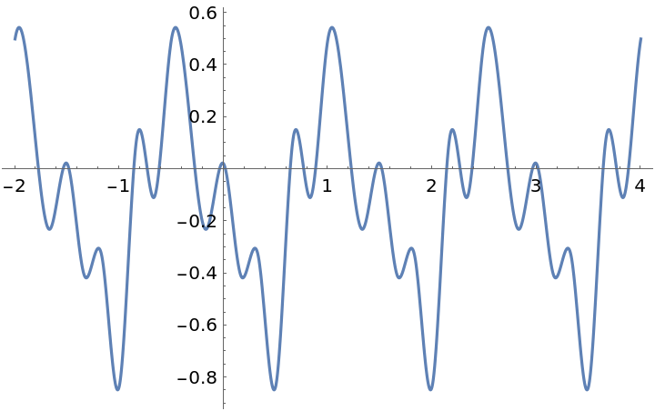
![fun = ResourceFunction["CubicSplineInterpolation"][
RandomFunction[
BrownianBridgeProcess[{1, 1/2}, {5/2, 1/2}], {1, 5/2, 1/6}][
"Path"], "Periodic"];
Plot[fun[x], {x, -2, 4}]](https://www.wolframcloud.com/obj/resourcesystem/images/481/4810d2d8-5392-4402-8a12-f378111551f4/378a6423af0d2b33.png)
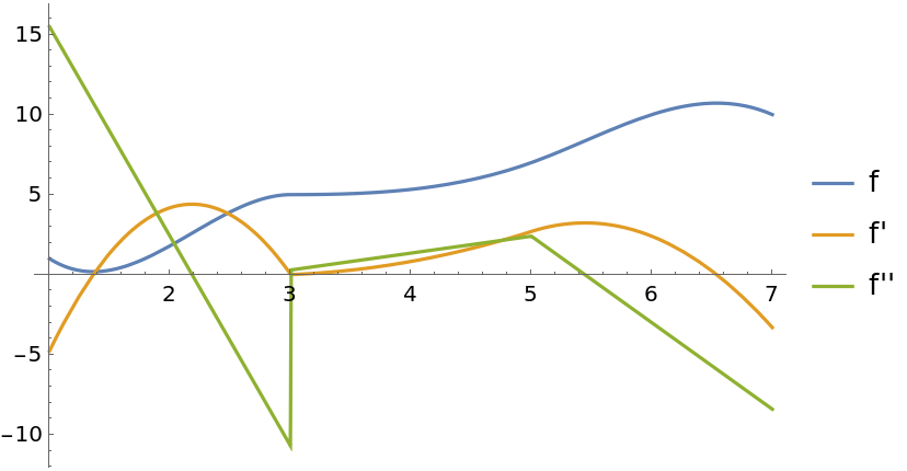
![data = {{1., 1.}, {2., 1.8}, {3., 5.}, {3.006, 5.0001}, {5., 7.}, {6.,
10.}, {7., 10.}};
fun = ResourceFunction["CubicSplineInterpolation"][data];
Plot[{fun[x], fun'[x], fun''[x]}, {x, 1, 7}, PlotLegends -> {"f", "f'", "f''"}, PlotRange -> All]](https://www.wolframcloud.com/obj/resourcesystem/images/481/4810d2d8-5392-4402-8a12-f378111551f4/50ffbe4ebf6577f8.png)