Wolfram Function Repository
Instant-use add-on functions for the Wolfram Language
Function Repository Resource:
Interpolate data with a monotonic piecewise cubic Hermite interpolant
ResourceFunction["CubicMonotonicInterpolation"][{f1,f2,…}] constructs a monotonic cubic Hermite interpolation of the function values fi, assumed to correspond to x values 1, 2, …. | |
ResourceFunction["CubicMonotonicInterpolation"][{{x1,f1},{x2,f2},…}] constructs a monotonic cubic Hermite interpolation of the function values fi corresponding to x values xi. |
Construct an approximate function that interpolates the data:
| In[1]:= |
| Out[1]= |
Apply the function to find interpolated values:
| In[2]:= |
| Out[2]= |
Plot the interpolation function along with the original data:
| In[3]:= |
| Out[3]= | 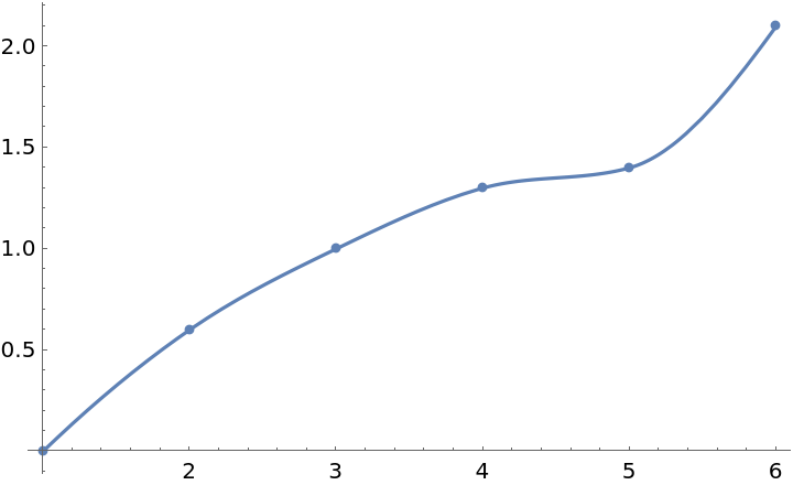 |
Interpolate and plot a monotonic data set:
| In[4]:= |
| Out[4]= |
| In[5]:= |
| Out[5]= | 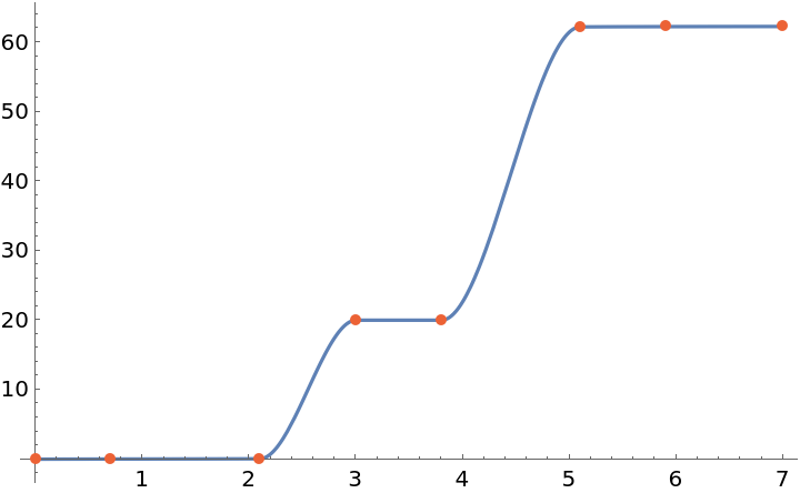 |
Form an interpolation from data given as a TimeSeries:
| In[6]:= |
| In[7]:= |
| Out[7]= | 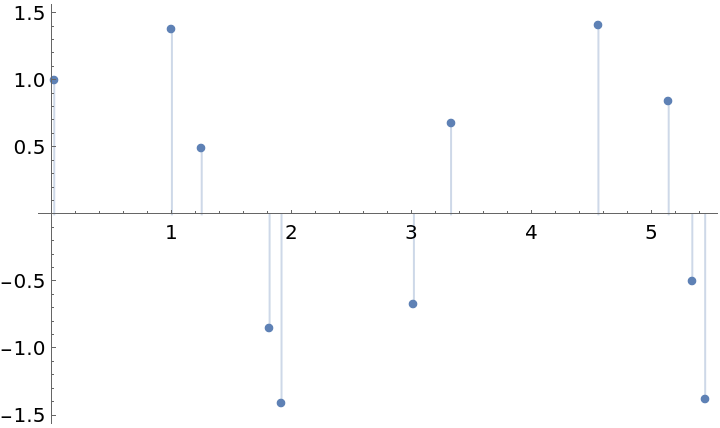 |
| In[8]:= |
| Out[8]= |
| In[9]:= |
| Out[9]= | 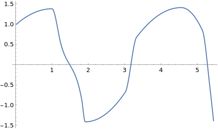 |
Compare different monotonic interpolation methods:
| In[10]:= |
| In[11]:= | ![fSte = ResourceFunction["CubicMonotonicInterpolation"][data, Method -> "Steffen"];
fFC = ResourceFunction["CubicMonotonicInterpolation"][data, Method -> "FritschCarlson"];
fSti = ResourceFunction["CubicMonotonicInterpolation"][data, Method -> "Stineman"];](https://www.wolframcloud.com/obj/resourcesystem/images/157/15779973-0285-4c3b-8cbd-d925e523396a/7559a0d2ec02050d.png) |
| In[12]:= |
| Out[12]= | 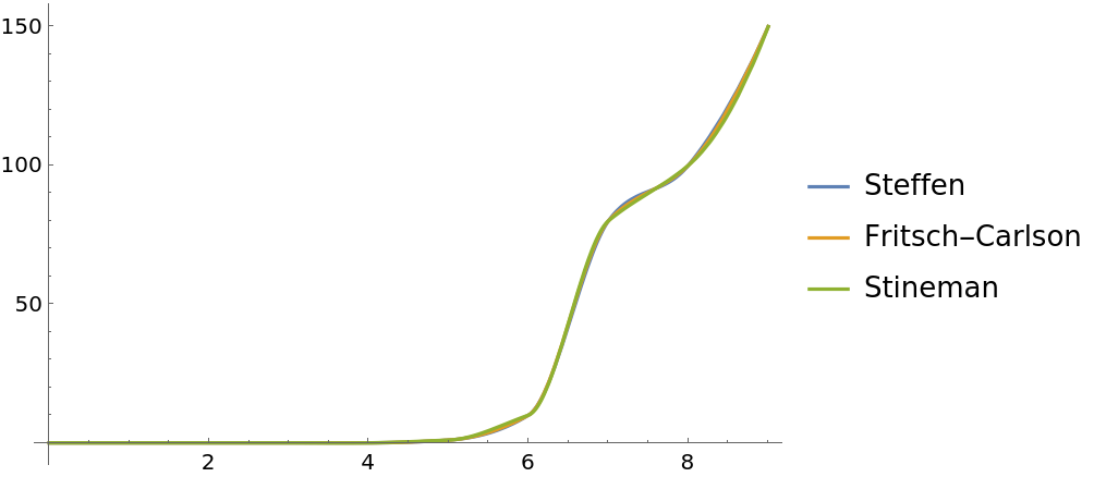 |
With PeriodicInterpolation->True, the data is interpreted as one period of a periodic function:
| In[13]:= |
| Out[13]= |
| In[14]:= |
| Out[14]= | 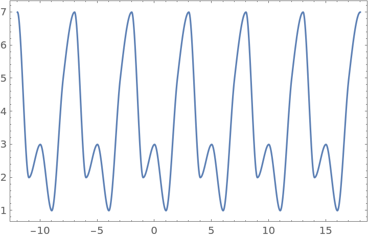 |
A monotonic data set:
| In[15]:= |
| In[16]:= | ![fHerm = Interpolation[data, Method -> "Hermite"];
fSpl = Interpolation[data, Method -> "Spline"];
fMon = ResourceFunction["CubicMonotonicInterpolation"][data];](https://www.wolframcloud.com/obj/resourcesystem/images/157/15779973-0285-4c3b-8cbd-d925e523396a/2142e90678a81cbd.png) |
Compare CubicMonotonicInterpolation with the built-in "Hermite" and "Spline" methods of Interpolation. The built-in methods do not preserve monotonicity, and give spurious oscillations:
| In[17]:= | ![Plot[{fMon[x], fHerm[x], fSpl[x]}, {x, 0, 1}, Epilog -> {Directive[AbsolutePointSize[5], ColorData[97, 4]], Point[data]}, PlotLegends -> {"Monotonic", "Hermite", "Spline"}, PlotRange -> All]](https://www.wolframcloud.com/obj/resourcesystem/images/157/15779973-0285-4c3b-8cbd-d925e523396a/1fe32329ab6f81e4.png) |
| Out[17]= | 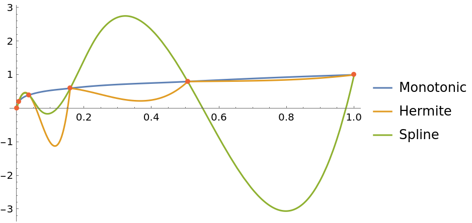 |
The interpolant returned by CubicMonotonicInterpolation is continuous up to its first derivative:
| In[18]:= |
| In[19]:= |
| Out[19]= | 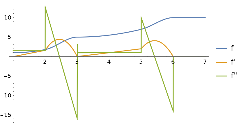 |
This work is licensed under a Creative Commons Attribution 4.0 International License