Wolfram Function Repository
Instant-use add-on functions for the Wolfram Language
Function Repository Resource:
Interpolate data using Akima's method or modifications of it
ResourceFunction["GeneralizedAkimaInterpolation"][{f1,f2,…}] constructs a cubic Hermite interpolation of the function values fi, assumed to correspond to x values 1, 2, …, using Akima's method. | |
ResourceFunction["GeneralizedAkimaInterpolation"][{{x1,f1},{x2,f2},…}] constructs a cubic Hermite interpolation of the function values fi corresponding to x values xi using Akima's method. |
| "AkimaClassic" | classical Akima method (1970) |
| "AkimaNew" | new Akima method (1991) |
| "ModifiedAkima" | Ionita's modification of Akima's method |
Construct an approximate function that interpolates the data:
| In[1]:= |
| Out[1]= |
Apply the function to find interpolated values:
| In[2]:= |
| Out[2]= |
Plot the interpolation function along with the original data:
| In[3]:= |
| Out[3]= | 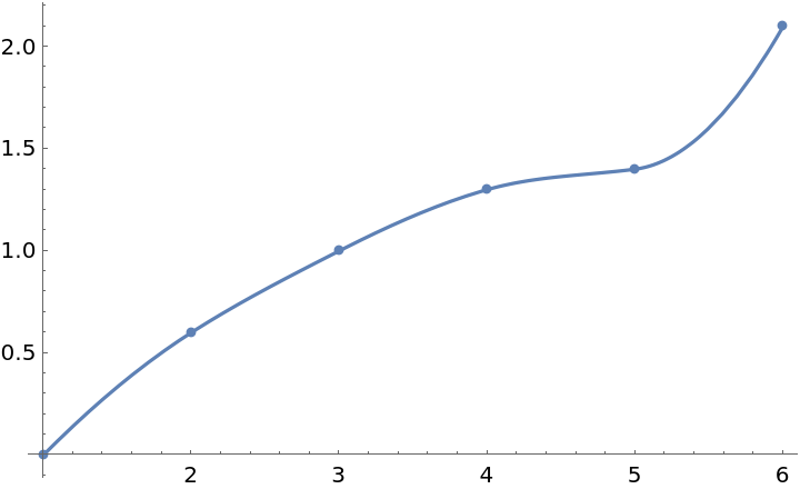 |
Interpolate between points at arbitrary x values:
| In[4]:= |
| In[5]:= |
| Out[5]= | 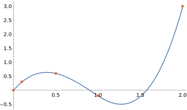 |
Form an interpolation from data given as a TimeSeries:
| In[6]:= |
| In[7]:= |
| Out[7]= |  |
| In[8]:= |
| Out[8]= |
| In[9]:= |
| Out[9]= | 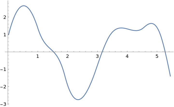 |
Compare different versions of Akima interpolation:
| In[10]:= |
| In[11]:= | ![f1970 = ResourceFunction["GeneralizedAkimaInterpolation"][data, Method -> "AkimaClassic"];
f1991 = ResourceFunction["GeneralizedAkimaInterpolation"][data, Method -> "AkimaNew"];
fMod = ResourceFunction["GeneralizedAkimaInterpolation"][data, Method -> "ModifiedAkima"];](https://www.wolframcloud.com/obj/resourcesystem/images/ef6/ef6cb7df-0097-46ca-ae8c-7f3f0b29d8af/2df97a2d3f420c9b.png) |
| In[12]:= |
| Out[12]= | 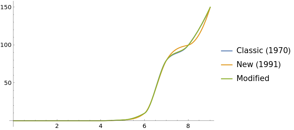 |
With PeriodicInterpolation→True, the data is interpreted as one period of a periodic function:
| In[13]:= |
| Out[13]= |
| In[14]:= |
| Out[14]= | 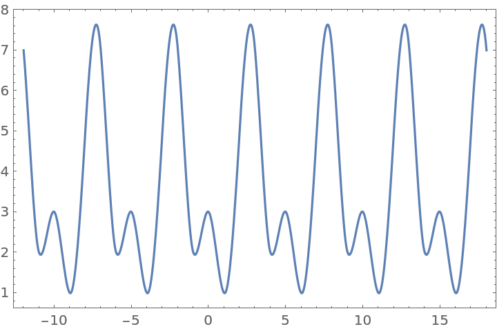 |
Setting Method→"AkimaClassic" in GeneralizedAkimaInterpolation gives results equivalent to the one from the resource function AkimaInterpolation:
| In[15]:= | ![data = {{1., 0.}, {2., 0.}, {3., 0.}, {4., 0.5}, {5., 0.4}, {5.5, 1.2}, {7., 1.2}, {8., 0.1}, {9., 0.}, {9.5, 0.3}, {10., 0.6}};
f1 = ResourceFunction["AkimaInterpolation"][data];
f2 = ResourceFunction["GeneralizedAkimaInterpolation"][data, Method -> "AkimaClassic"];](https://www.wolframcloud.com/obj/resourcesystem/images/ef6/ef6cb7df-0097-46ca-ae8c-7f3f0b29d8af/2df3a19fed922cf3.png) |
| In[16]:= |
| Out[16]= |  |
The interpolant returned by GeneralizedAkimaInterpolation is continuous up to its first derivative:
| In[17]:= |
| In[18]:= |
| Out[18]= | 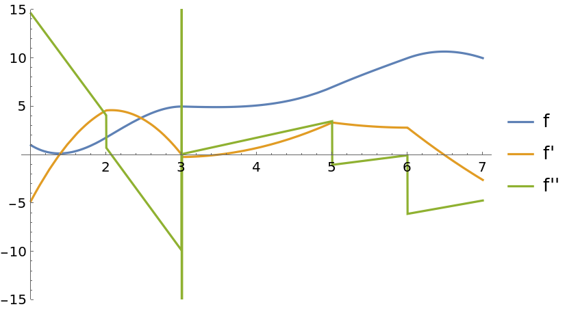 |
This work is licensed under a Creative Commons Attribution 4.0 International License