Function Repository Resource:

ArcInterpolation

Source Notebook

Create an interpolation augmented with first derivatives of circles through consecutive point triples

Contributed by: Robert Rimmer

ResourceFunction["ArcInterpolation"][{{x₁,f₁},{x₂,f₂},…}]

constructs an interpolation of the function values f_i corresponding to values x_i.

Details and Options

The input must be a list of {x,y} pairs of real numbers.

The interpolations are smoother when the data is ordered by x_i.

ResourceFunction["ArcInterpolation"] uses Interpolation and returns an InterpolatingFunction object.

ResourceFunction["ArcInterpolation"] adds a first derivative for each midpoint of sequential three points, calculated using CircleThrough on the three points. It returns Automatic if there would be a division by zero error.

ResourceFunction["ArcInterpolation"] has an option "Endpoints" (default False), which, when set to True, which will calculate the slope of the first and last points from the second and penultimate circles.

It passes on relevant options such as InterpolationOrder to Interpolation (although Method→"Spline" is not supported because derivatives are being used).

Examples

Basic Examples (2)

Create an arc interpolation for some points:

In[1]:=

Out[1]=

Compare the fit by ArcInterpolation (orange) to a simple data set with the fit by Interpolation:

In[2]:=

data = {{1, 1}, {2, 2}, {3, 3}, {4, 5}, {5, 8}, {6, 5}};
ifn = Interpolation[data];
afn = ResourceFunction["ArcInterpolation"][data];
Plot[{ifn[x], afn[x]}, {x, 1, 6}, PlotLegends -> {"Interpolation", "ArcInterpolation"}, Epilog -> Point@data]

Out[5]=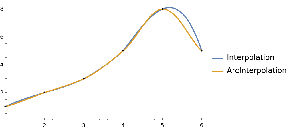

First derivatives are smoother, because a first derivative has been given to Interpolation:

In[6]:=

Out[6]=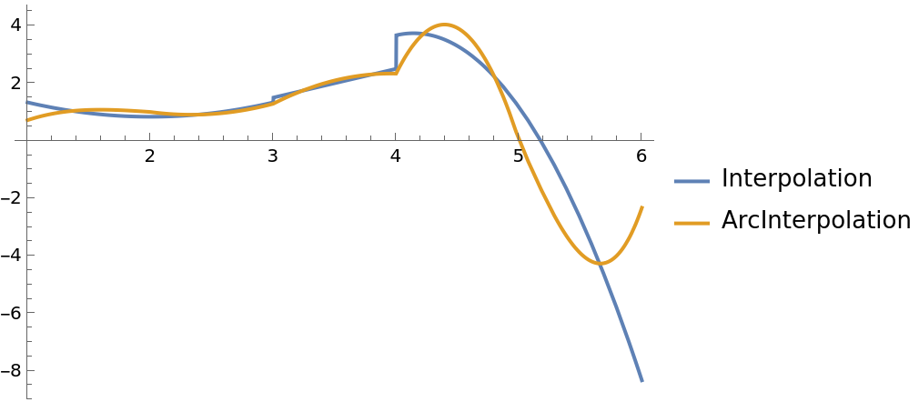

Scope (6)

The strategy for ArcInterpolation was developed to deal with inverted treasury yield curves, which cannot be well fit with Interpolation. Define data:

In[7]:=

yc = {{1/13, 5.53`}, {2/13, 5.56`}, {1/4, 5.53`}, {17/52, 5.5`}, {1/2,
5.45`}, {1, 5.29`}, {2, 4.83`}, {3, 4.62`}, {5, 4.49`}, {7, 4.55`}, {10, 4.57`}, {20, 4.93`}, {30, 4.77`}}

Out[7]=

Create interpolations of various orders with Interpolation and ArcInterpolation:

In[8]:=

Out[8]=

In[9]:=

Out[9]=

The standard third order Interpolation has an erratic shape compared to ArcInterpolation:

In[10]:=

Plot[Evaluate[(#[[2]][t]) & /@ {ycurves, aycurves}], {t, 1/13, 30}, PlotRange -> All, PlotLegends -> {"Interpolation", "ArcInterpolation"}, PlotLabel -> "Third Order Interpolation", Epilog -> Point@yc]

Out[10]=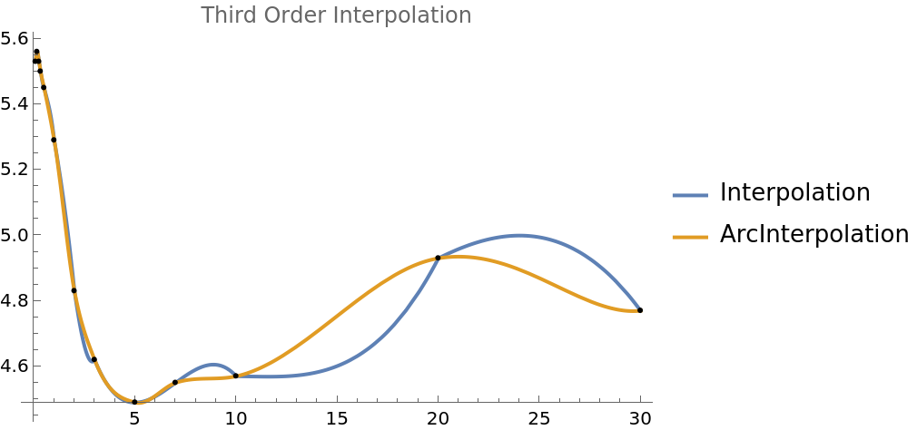

Second order is a little better for Interpolation, but it still has an erratic shape at t=20:

In[11]:=

Plot[Evaluate[(#[[1]][t]) & /@ {ycurves, aycurves}], {t, 1/13, 30}, PlotRange -> All, PlotLegends -> {"Interpolation", "ArcInterpolation"}, PlotLabel -> "Second Order Interpolation", Epilog -> Point@yc]

Out[11]=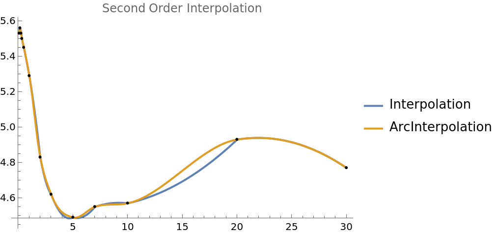

Fourth order is useless in this case for Interpolation, but an acceptable choice for ArcInterpolation:

In[12]:=

Plot[Evaluate[(#[[3]][t]) & /@ {ycurves, aycurves}], {t, 1/13, 30}, PlotRange -> All, PlotLegends -> {"Interpolation", "ArcInterpolation"}, PlotLabel -> "Fourth Order Interpolation", Epilog -> Point@yc]

Out[12]=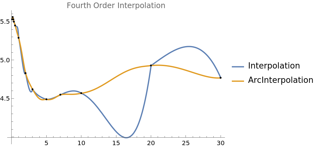

The option setting "Endpoints"→True changes the shape of the yield curve, extending a circular shape from the point at t=20:

In[13]:=

ycfn = ResourceFunction["ArcInterpolation"][yc];
ycfne = ResourceFunction["ArcInterpolation"][yc, "Endpoints" -> True];
Plot[{ycfn[t], ycfne[t]}, {t, 1/13, 30}]

Out[14]=

Properties and Relations (5)

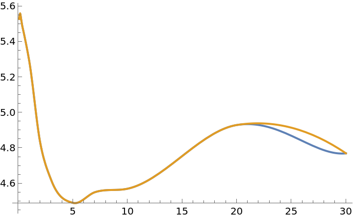ArcInterpolation makes no assumptions about monotonicity. This is an example from the resource function MonotonicInterpolation to compare fits to data. ArcInterpolation preserves the monotonicity of the data, but moves the bends in the functions to the node points:

In[15]:=

data = {{0.0, 0.0}, {0.7, 0.02}, {2.1, 0.06}, {3.0, 8.28}, {3.8, 57.6}, {5.1, 62.2}, {5.9, 62.24}, {7.0, 62.26}};
afn3 = ResourceFunction["ArcInterpolation"][data];
MonotonicInterpolation = ResourceFunction["MonotonicInterpolation"];
fun = MonotonicInterpolation[data];
Plot[{afn3[x], fun[x]}, {x, 0, 7}, Epilog -> Point@data]

Out[16]=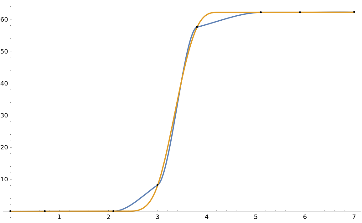

Here is a more complicated example from the resource function CubicMonotonicInterpolation:

In[17]:=

ts = TemporalData[
TimeSeries, {{{1, Cos[1] + Sin[1], Cos[2] + Sin[2], Cos[3] + Sin[3],
Cos[4] + Sin[4], Cos[5] + Sin[5], Cos[6] + Sin[6], Cos[7] + Sin[7], Cos[8] + Sin[8], Cos[9] + Sin[9], Cos[10] + Sin[10]}}, {{{0.016965744360214943`, 0.9973865299845299, 1.24591736467102, 1.8114088692820352`, 1.9107450982712126`, 3.013995043949912, 3.323754146542503, 4.551557869716615, 5.13709169763333, 5.334143602077121, 5.441221219515277}}}, 1, {"Continuous", 1}, {"Discrete", 1}, 1, {ResamplingMethod -> {"Interpolation", InterpolationOrder -> 1}}},
False, 10.1];
ListPlot[ts, Filling -> Axis]

Out[18]=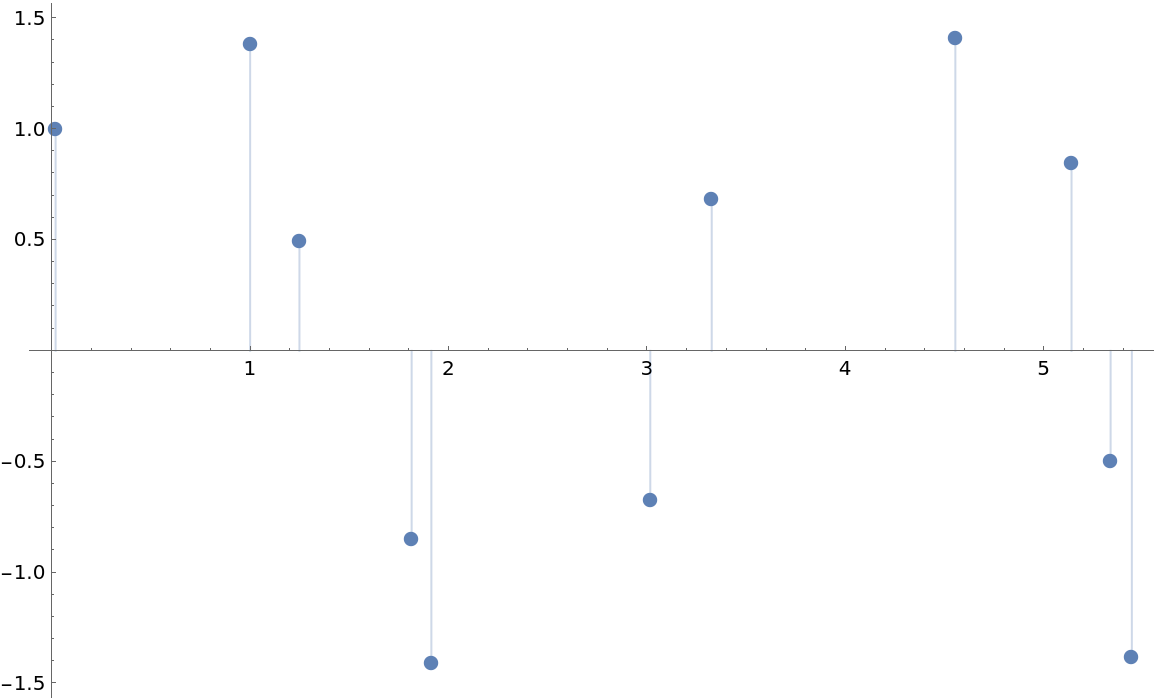

Here the ArcInterpolation function does not find monotonicity in the first two data points, but if it uses the end point slope extrapolated from the second data point circle then it avoids an extreme oscillation:

In[19]:=

fun = ResourceFunction["CubicMonotonicInterpolation"][ts];
afn1 = ResourceFunction["ArcInterpolation"][Normal@ts, "Endpoints" -> True];
afn2 = ResourceFunction["ArcInterpolation"][Normal@ts];
Plot[{afn1[x], afn2[x], fun[x]}, {x, ts["FirstTime"], ts["LastTime"]},
Epilog -> Point@Normal[ts]]

Out[20]=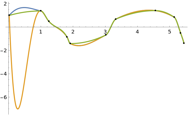

The recent yield curve is not monotonic, but the fit to CubicMonotonicInterpolation is similar if the "Endpoints" are included:

In[21]:=

yc = {{1/13, 5.53`}, {2/13, 5.56`}, {1/4, 5.53`}, {17/52, 5.5`}, {1/2,
5.45`}, {1, 5.29`}, {2, 4.83`}, {3, 4.62`}, {5, 4.49`}, {7, 4.55`}, {10, 4.57`}, {20, 4.93`}, {30, 4.77`}};
ycfn = ResourceFunction["ArcInterpolation"][yc, "Endpoints" -> True];
cmfn = ResourceFunction["CubicMonotonicInterpolation"][yc];
Plot[{ycfn[t], cmfn[t]}, {t, 1/13, 30}]

Out[22]=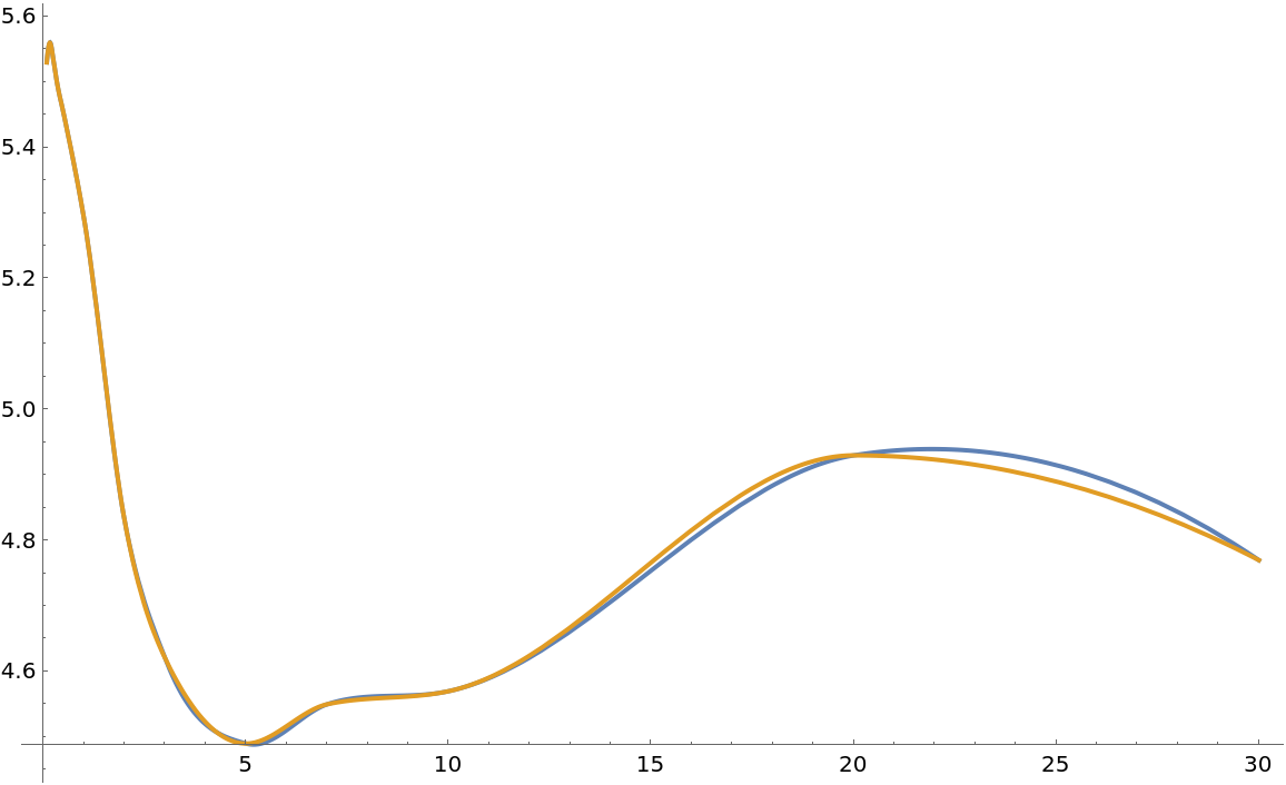

CubicMontonicInterpolation also supports Method→"Stineman", which gives close to the same result by using a circular derivative:

In[23]:=

Out[24]=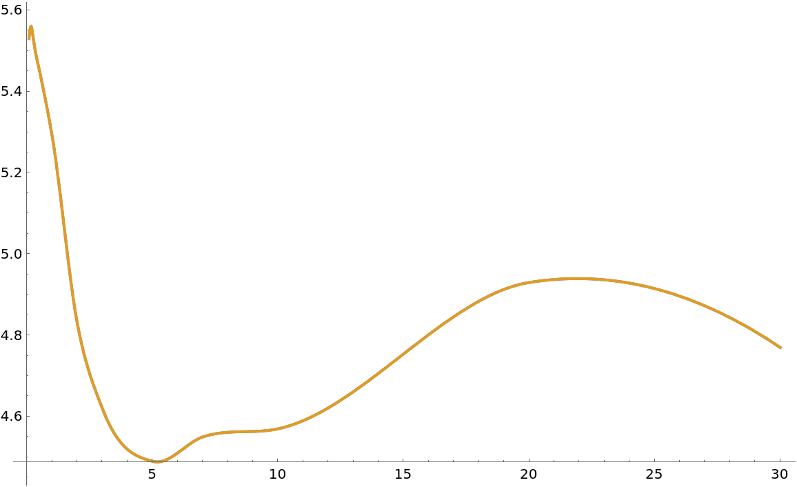

In[25]:=

Out[25]=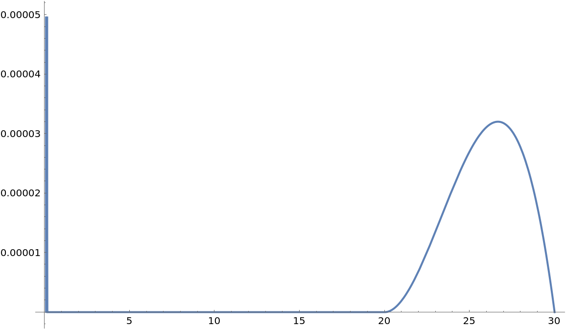

Neat Examples (1)

In[26]:=

Circles through three points sequentially are shown with the points and fit to the curve:

In[27]:=

circ = CircleThrough /@ Partition[yc, 3, 1];
ycfn = ResourceFunction["ArcInterpolation"][yc];
Show[Plot[ycfn[t], {t, 1/13, 30}, PlotRange -> {{1/13, 31}, {0, 6}}, PlotStyle -> {Red, Thick}], Graphics[{Blue, circ}], ListPlot[yc, PlotStyle -> Black], ImageSize -> 600]

Out[29]=

Publisher

Robert Rimmer

Requirements

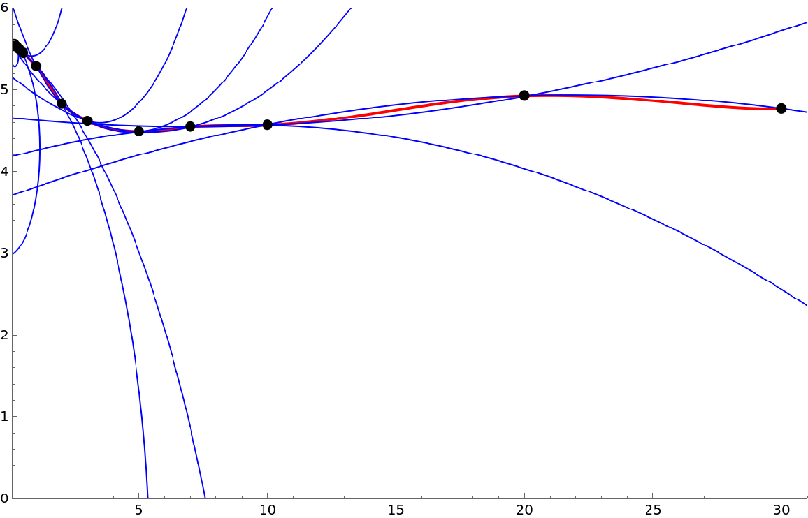Wolfram Language 13.0 (December 2021) or above

Version History

1.0.0 – 06 December 2023

Related Resources

Author Notes

The strategy behind ArcInterpolation is rather simple compared to other interpolation methods. A circle can be fit to any three points, which are not collinear, on a plane. The lowest order univariate polynomial which can be fit to three points is a quadratic parabola. This function however is constrained by being symmetric in curvature to a line through the vertex parallel to the y-axis. Further the slope of a quadratic parabola is always zero at the vertex, and the degree of its curvature diminishes with distance from the vertex axis, so its behavior is biased to the Cartesian coordinate system. A circle has no such constraints and its curvature is symmetric about its radius to any point on the circle. In the case of the yield curve examples, choosing circular slopes tends to shift more dramatic changes in slope of the function to the node points. Thus it may be useful for data functions where the node points are chosen because they are special. This is the case for the yield curve the node points, which are chosen to match the maturities of bills and notes issued by the Treasury. Consequently there is heavier trading in these maturities, and they have more influence on the yield curve function.

License Information

This work is licensed under a Creative Commons Attribution 4.0 International License