Wolfram Research

Function Repository Resource:

AkimaInterpolation (1.0.0) current version: 1.0.1 »

Source Notebook

Interpolation and smooth curve fitting based on local procedures

Contributed by: Robert B. Nachbar (Wolfram Solutions)

ResourceFunction["AkimaInterpolation"][{f1,f2,}]

constructs an interpolation of the function values fi, assumed to correspond to x values of 1,2,, using Akima’s method.

ResourceFunction["AkimaInterpolation"][{{x1,f1},{x2,f2},}]

constructs an interpolation of the function values fi corresponding to x values xi.

Details and Options

ResourceFunction["AkimaInterpolation"] returns an InterpolatingFunction object, which can be used like any other pure function.
The interpolation function returned by ResourceFunction["AkimaInterpolation"][data] is set up so as to agree with data at every point explicitly specified in data.
The function values fi are expected to be real or complex numbers.
The function arguments xi must be real numbers.
The interpolation works by fitting a third-degree polynomial curve between successive data points.
The interpolation automatically makes use of local numerical derivatives.
If the data is periodic, only the data for a single fundamental period are required. The option PeriodicInterpolation is used.

Examples

Basic Examples (4) 

Construct an approximate function that interpolates the data:

In[1]:=
f = ResourceFunction["AkimaInterpolation"][{1, 2, 3, 5, 8, 5}]
Out[1]=

Apply the function to find interpolated values :

In[2]:=
f[2.5]
Out[2]=

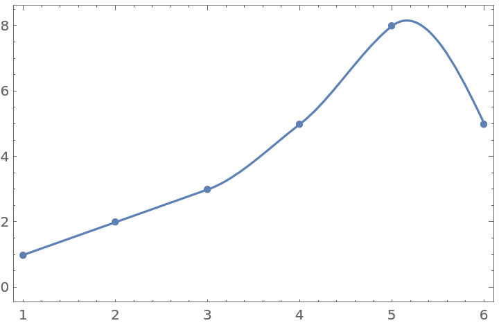
Plot the interpolation function:

In[3]:=
Plot[f[x], {x, 1, 6}]
Out[3]=

Compare with the original data:

In[4]:=
Show[%, ListPlot[{1, 2, 3, 5, 8, 5}]]
Out[4]=

Scope (1) 

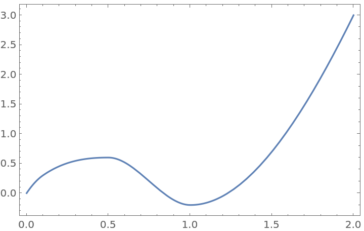
Interpolate between points at arbitrary x-values:

In[5]:=
ResourceFunction["AkimaInterpolation", ResourceVersion->"1.0.0"][{{0, 0}, {0.1, .3}, {0.5, .6}, {1, -.2}, {2, 3}}]
Out[5]=
In[6]:=
Plot[%[x], {x, 0, 2}]
Out[6]=

Options (1) 

PeriodicInterpolation (1) 

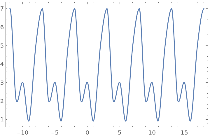
With PeriodicInterpolationTrue, the data is interpreted as one period of a periodic function:

In[7]:=
fp = ResourceFunction["AkimaInterpolation"][{1, 5, 7, 2, 3, 1}, PeriodicInterpolation -> True]
Out[7]=
In[8]:=
Plot[fp[x], {x, -12, 18}]
Out[8]=

Applications (1) 

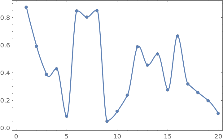
Interpolate random data:

In[9]:=
f = ResourceFunction["AkimaInterpolation"][r = RandomReal[1, 20]]
Out[9]=
In[10]:=
Show[ListPlot[r], Plot[f[x], {x, 1, 20}]]
Out[10]=

Properties and Relations (2) 

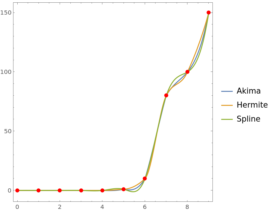
Compare the output from AkimaInterpolation to that from Interpolation:

In[11]:=
data = {{0, 0}, {1, 0}, {2, 0}, {3, 0}, {4, 0}, {5, 1}, {6, 10}, {7, 80}, {8, 100}, {9, 150}};
afun = ResourceFunction["AkimaInterpolation"][data];
ifun = Interpolation[data];
sfun = Interpolation[data, Method -> Spline];
In[12]:=
Plot[{ifun[x], afun[x], sfun[x]}, {x, 0, 9}, Epilog -> {Red, PointSize[0.02], Point[data]}, PlotLegends -> {"Akima", "Hermite", "Spline"}, AspectRatio -> 1]
Out[12]=

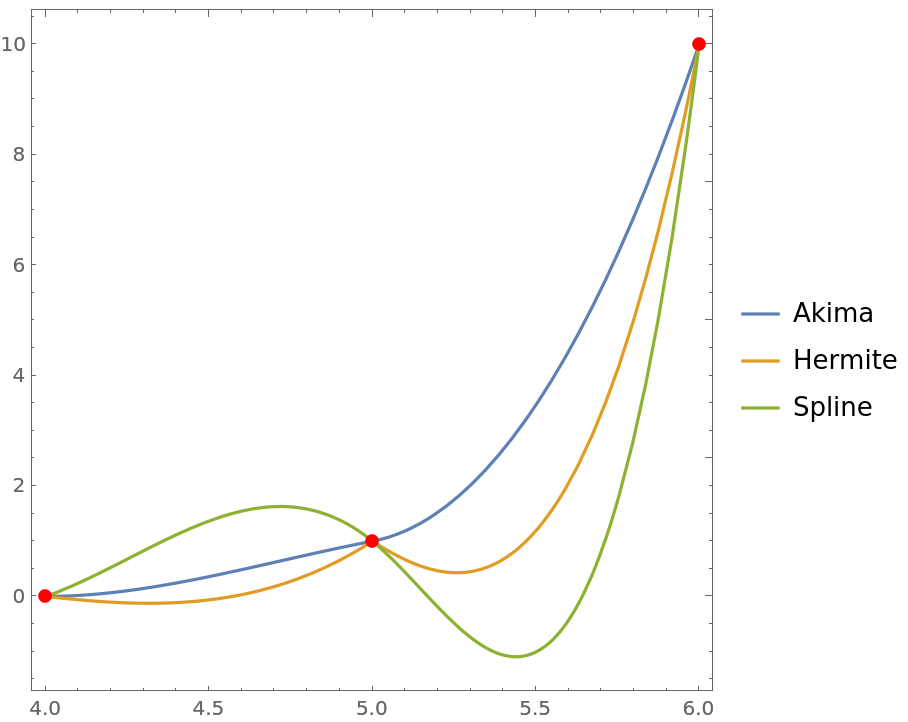
Examine the region between 4 and 6:

In[13]:=
Plot[{afun[x], ifun[x], sfun[x]}, {x, 4, 6}, Epilog -> {Red, PointSize[0.02], Point[data]}, PlotLegends -> {"Akima", "Hermite", "Spline"}, AspectRatio -> 1]
Out[13]=

Possible Issues (3) 

Extrapolation is attempted to go beyond the original data:

In[14]:=
f = ResourceFunction["AkimaInterpolation"][{1, 2, 4, -2, 1}]
Out[14]=
In[15]:=
Table[f[i], {i, 0, 6}]
Out[15]=

At least 2 points are needed:

In[16]:=
ResourceFunction["AkimaInterpolation"][{1}]
Out[16]=
In[17]:=
ResourceFunction["AkimaInterpolation"][{1, 2}]
Out[17]=

The interpolation function will always be continuous and first-order differentiable, but may not be higher-order differentiable:

In[18]:=
f = ResourceFunction["AkimaInterpolation"][r = RandomReal[1, 10]]
Out[18]=
In[19]:=
Show[Plot[Evaluate[{f[x], D[f[x], x], D[f[x], {x, 2}]}], {x, 1, 10}, PlotLegends -> {\[ScriptF], Derivative[1][\[ScriptF]][x], (\[ScriptF]^\[Prime]\[Prime])[x]}], ListPlot[r]]
Out[19]=

Neat Examples (2) 

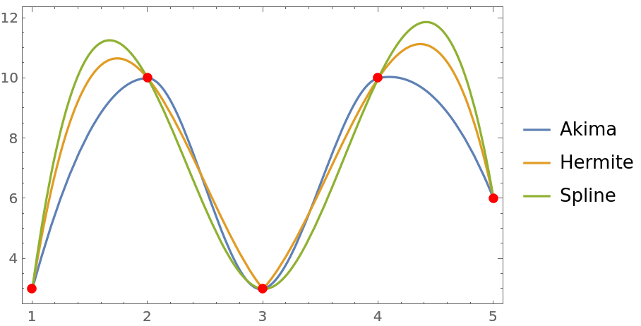
Excessive undulation is suppressed:

In[20]:=
data = {3, 10, 3, 10, 6};
afun = ResourceFunction["AkimaInterpolation"][data];
ifun = Interpolation[data];
sfun = Interpolation[data, Method -> "Spline"];
Plot[{afun[x], ifun[x], sfun[x]}, {x, 1, 5}, Epilog -> {Red, PointSize[0.02], Point[Thread[{Range[5], data}]]}, PlotLegends -> {"Akima", "Hermite", "Spline"}]
Out[20]=

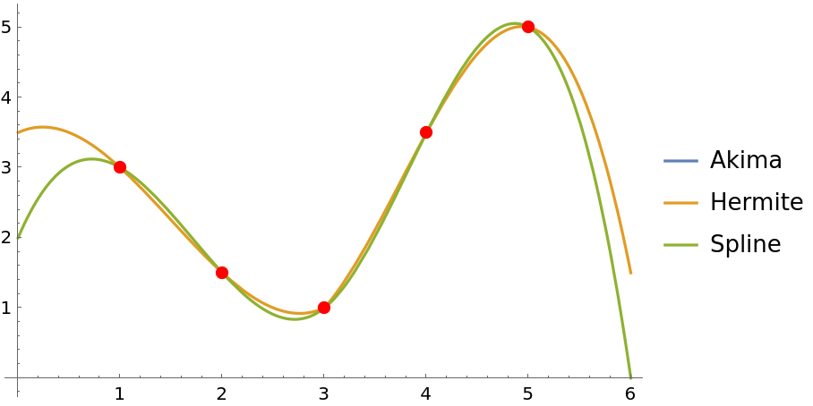
Reasonable extrapolation is permitted:

In[21]:=
data = {{1, 3}, {2, 3/2}, {3, 1}, {4, 7/2}, {5, 5}};
afun = ResourceFunction["AkimaInterpolation"][data];
ifun = Interpolation[data];
sfun = Interpolation[data, Method -> "Spline"];
Plot[{afun[x], ifun[x], sfun[x]}, {x, 0, 6}, Epilog -> {Red, PointSize[0.02], Point[data]}, PlotLegends -> {"Akima", "Hermite", "Spline"}]
Out[22]=

Publisher

Robert Nachbar

Requirements

Wolfram Language 11.3 (March 2018) or above

Version History

  • 1.0.1 – 24 January 2024
  • 1.0.0 – 09 January 2019

Source Metadata

Related Resources

License Information