Wolfram Function Repository
Instant-use add-on functions for the Wolfram Language
Function Repository Resource:
Interpolation and smooth curve fitting based on local procedures
ResourceFunction["AkimaInterpolation"][{f1,f2,…}] constructs an interpolation of the function values fi, assumed to correspond to x values of 1,2,…, using Akima’s method. | |
ResourceFunction["AkimaInterpolation"][{{x1,f1},{x2,f2},…}] constructs an interpolation of the function values fi corresponding to x values xi. |
Construct an approximate function that interpolates the data:
| In[1]:= |
| Out[2]= |
Apply the function to find interpolated values:
| In[3]:= |
| Out[3]= |
Plot the interpolation function:
| In[4]:= |
| Out[4]= | 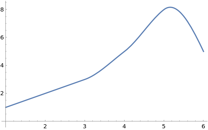 |
Compare with the original data:
| In[5]:= |
| Out[5]= | 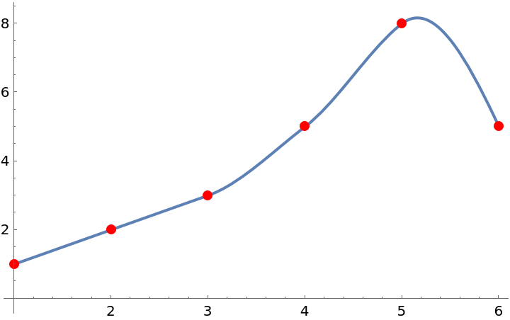 |
Interpolate between points at arbitrary x-values:
| In[6]:= |
| Out[6]= |
| In[7]:= |
| Out[7]= | 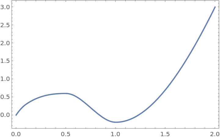 |
With PeriodicInterpolation→True, the data are interpreted as one period of a periodic function:
| In[8]:= |
| Out[9]= |
Periodic interpolation can be used outside the range of the data:
| In[10]:= |
| Out[10]= | 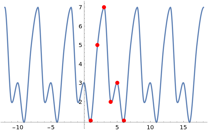 |
Interpolate random data:
| In[11]:= |
| Out[11]= |
| In[12]:= |
| Out[12]= | 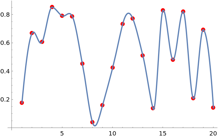 |
Compare the output from AkimaInterpolation to that from Interpolation:
| In[13]:= | ![data = {{0, 0}, {1, 0}, {2, 0}, {3, 0}, {4, 0}, {5, 1}, {6, 10}, {7, 80}, {8, 100}, {9, 150}};
afun = ResourceFunction["AkimaInterpolation"][data];
ifun = Interpolation[data];
sfun = Interpolation[data, Method -> Spline];
Plot[{ifun[x], afun[x], sfun[x]}, {x, 0, 9}, Epilog -> {Red, PointSize[0.02], Point[data]}, PlotLegends -> {"Akima", "Hermite", "Spline"}, AspectRatio -> 1]](https://www.wolframcloud.com/obj/resourcesystem/images/80d/80ddd816-2854-426d-bb20-fb42f5f55c82/2a604d148230c1ba.png) |
| Out[14]= | 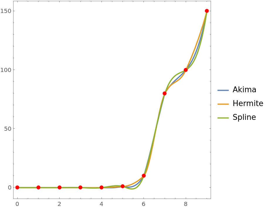 |
Examine the region between 4 and 6:
| In[15]:= |
| Out[15]= | 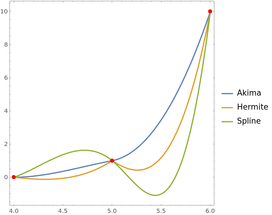 |
Extrapolation is attempted to go beyond the original data:
| In[16]:= |
| Out[16]= |
| In[17]:= |
| Out[17]= |
At least 2 points are needed:
| In[18]:= |
| Out[18]= |
| In[19]:= |
| Out[19]= |
The interpolation function will always be continuous and first-order differentiable, but may not be higher-order differentiable:
| In[20]:= |
| Out[20]= |
| In[21]:= | ![Show[Plot[Evaluate[{f[x], D[f[x], x], D[f[x], {x, 2}]}], {x, 1, 10}, PlotLegends -> {\[ScriptF], Derivative[1][\[ScriptF]][x], (\[ScriptF]^\[Prime]\[Prime])[x]}], ListPlot[r, PlotStyle -> {PointSize[Large], Red}]]](https://www.wolframcloud.com/obj/resourcesystem/images/80d/80ddd816-2854-426d-bb20-fb42f5f55c82/27f552b14b2527d1.png) |
| Out[21]= | 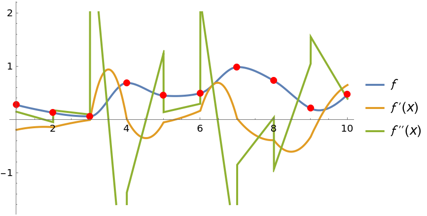 |
Excessive undulation is suppressed:
| In[22]:= | ![data = {3, 10, 3, 10, 6};
afun = ResourceFunction["AkimaInterpolation"][data];
ifun = Interpolation[data];
sfun = Interpolation[data, Method -> "Spline"];
Plot[{afun[x], ifun[x], sfun[x]}, {x, 1, 5}, Epilog -> {Red, PointSize[0.02], Point[Thread[{Range[5], data}]]}, PlotLegends -> {"Akima", "Hermite", "Spline"}]](https://www.wolframcloud.com/obj/resourcesystem/images/80d/80ddd816-2854-426d-bb20-fb42f5f55c82/4b9060cc2ed5ad27.png) |
| Out[23]= | 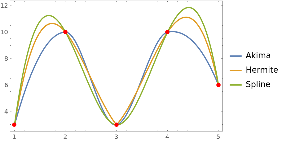 |
Reasonable extrapolation is permitted:
| In[24]:= | ![data = {{1, 3}, {2, 3/2}, {3, 1}, {4, 7/2}, {5, 5}};
afun = ResourceFunction["AkimaInterpolation"][data];
ifun = Interpolation[data];
sfun = Interpolation[data, Method -> "Spline"];
Plot[{afun[x], ifun[x], sfun[x]}, {x, 0, 6}, Epilog -> {Red, PointSize[0.02], Point[data]}, PlotLegends -> {"Akima", "Hermite", "Spline"}]](https://www.wolframcloud.com/obj/resourcesystem/images/80d/80ddd816-2854-426d-bb20-fb42f5f55c82/2c9a7b5f156af6b6.png) |
| Out[28]= | 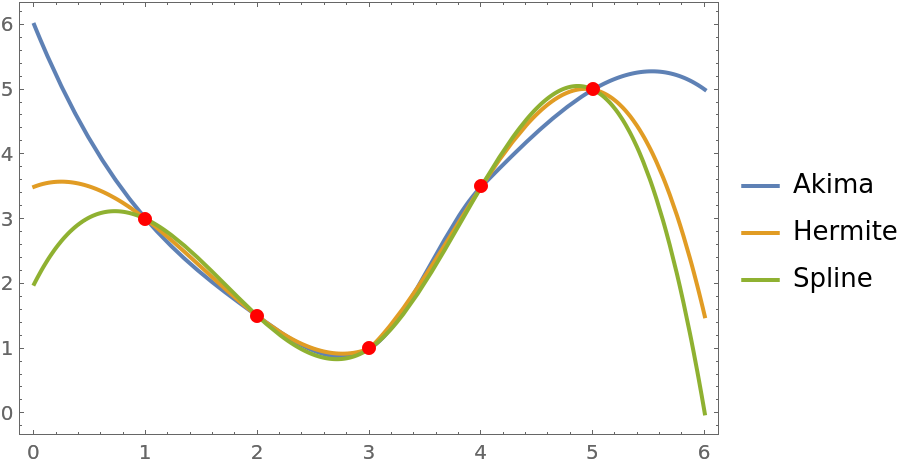 |
Wolfram Language 11.3 (March 2018) or above
This work is licensed under a Creative Commons Attribution 4.0 International License