Wolfram Language Paclet Repository

Community-contributed installable additions to the Wolfram Language

Primary Navigation

    • Cloud & Deployment
    • Core Language & Structure
    • Data Manipulation & Analysis
    • Engineering Data & Computation
    • External Interfaces & Connections
    • Financial Data & Computation
    • Geographic Data & Computation
    • Geometry
    • Graphs & Networks
    • Higher Mathematical Computation
    • Images
    • Knowledge Representation & Natural Language
    • Machine Learning
    • Notebook Documents & Presentation
    • Scientific and Medical Data & Computation
    • Social, Cultural & Linguistic Data
    • Strings & Text
    • Symbolic & Numeric Computation
    • System Operation & Setup
    • Time-Related Computation
    • User Interface Construction
    • Visualization & Graphics
    • Random Paclet
    • Alphabetical List
  • Using Paclets
    • Get Started
    • Download Definition Notebook
  • Learn More about Wolfram Language

TerraPercolatio

Guides

  • TerraPercolatio

Tech Notes

  • Solving Seepage Problems with TerraPercolatio

Symbols

  • BoundaryFlux
  • ExitGradient
  • FlowNet
  • PorePressureField
  • SeepagePlot
  • SeepageSolve
  • SeepageUnconfined
  • SeepageWell
  • TerraPercolatioClear
  • TerraPercolatio
Solving Seepage Problems with TerraPercolatio
Flow into a dewatered excavation behind sheet piles
3D flow into a rectangular excavation
Unconfined flow through a homogeneous earth dam
Parallel drainage trenches at a spacing (water-table lowering)
TerraLapsus slope: seepage through a 1:2 slope
Line of wellpoints at a spacing (excavation dewatering)
Axisymmetric flow to a pumped well (drawdown cone)
Working with the solution object
General 2D steady-state seepage solver: multi-layer anisotropic materials, confined and unconfined flow, true flow nets from the exact dual (stream-function) problem. Put TerraPercolatio.wl in the same directory as this notebook and evaluate the cells in order.
Flow into a dewatered excavation behind sheet piles
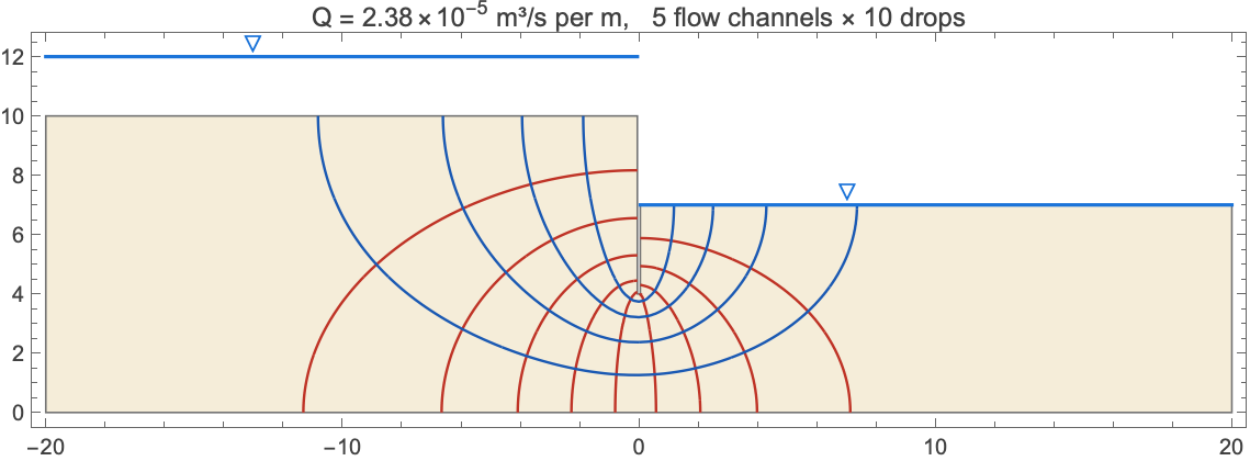
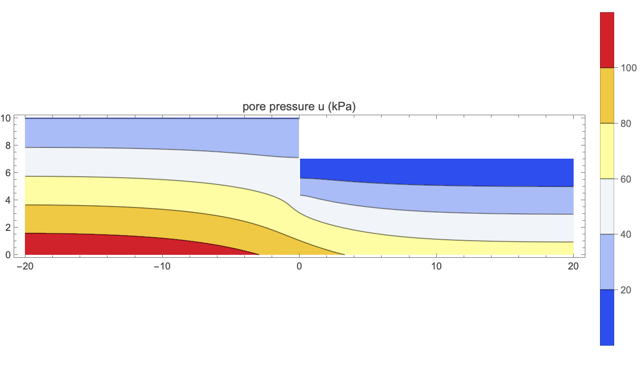
A sheet-pile wall (modelled as a thin slit) retains a 3 m deep excavation in a 10 m permeable stratum over an impermeable base. Upstream there are 2 m of standing water above ground level; downstream the ground is excavated to 7 m and dewatered, so the water level in the excavation coincides with the excavated ground level. All parameters are named below:
In[12]:=
gUp=10.;(*upstreamgroundlevel,m*)​​gExc=7.;(*excavatedgroundlevel=waterlevelintheexcavation,m*)​​hUp=12.;(*upstreamwaterlevel:2mstandingwateraboveground,m*)​​hDn=gExc;(*downstreamhead:excavationdewateredtofloorlevel,m*)​​ytip=4.;(*piletipelevation:6mbelowu/sground,3mbelowfloor,m*)​​w=0.05;(*half-thicknessofthepileslit,m*)​​L=20.;(*lateralextentofthemodeleithersideofthewall,m*)​​kSand=1.*^-5;(*isotropicpermeability,m/s*)​​​​excPoly={{-L,0.},{L,0.},{L,gExc},{w,gExc},{w,ytip},{-w,ytip},{-w,gUp},{-L,gUp}};​​excLayers={"Polygon"excPoly,"kx"kSand,"ky"kSand};​​excHeadBCs={{hUp,Function[{x,y},y≥gUp-10.^-6&&x≤-w]},(*u/sgroundsurface*){hDn,Function[{x,y},y≥gExc-10.^-6&&x≥w]}};(*excavationfloor*)​​pilePred=Function[{x,y},Abs[x]≤w+10.^-6&&y≥ytip-10.^-6];(*wall=streamline*)​​outerPred=Function[{x,y},y≤10.^-6||Abs[x]≥L-10.^-6];(*base&farfield*)excSol=
SeepageSolve
[excLayers,excHeadBCs,{pilePred,outerPred},"MeshSize"0.4];​​excSol["Q"]
Out[25]=
0.0000238332
The "WaterLevels" option draws free-water surfaces (with the ▽ symbol), including standing water above ground — here the 2 m of ponded water upstream and the water held at floor level in the excavation:
In[26]:=
FlowNet[excSol, "PotentialDrops" -> 10,
"WaterLevels" -> {{hUp, {-L, -w}}, {hDn, {w, L}}},
PlotRange -> {{-L - 0.5, L + 0.5}, {-0.5, 12.8}}, ImageSize -> 900]
Out[26]=
Exit gradient across the excavation floor next to the wall (piping/heave check — compare with icrit ≈ 1):
In[27]:=
ExitGradient[excSol, Function[{x, y}, y >= gExc - 10.^-3 && w + 0.01 <= x <= 3.]]
Out[27]=
0.427694
In[28]:=
SeepagePlot[excSol, "PorePressure", ImageSize -> 600]
Out[28]=

Same excavation, two-layer anisotropic soil

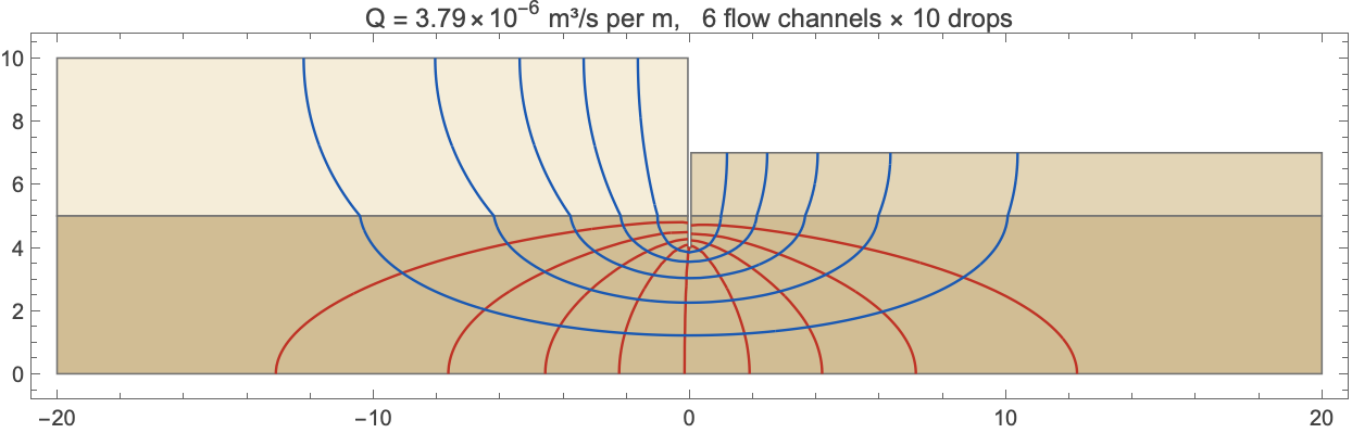
The stratum below 5 m is finer and anisotropic (kx = 2×10^-6, ky = 5×10^-7 m/s). Adjacent layer polygons must share vertices along interfaces; a layer interrupted by the wall is supplied as two polygons with the same k. Note the streamline refraction at the interface:
In[29]:=
yInt=5.;(*layerinterfaceelevation,m*)​​lowerP={{-L,0.},{L,0.},{L,yInt},{w,yInt},{w,ytip},{-w,ytip},{-w,yInt},{-L,yInt}};​​upLeft={{-L,yInt},{-w,yInt},{-w,gUp},{-L,gUp}};​​upRight={{w,yInt},{L,yInt},{L,gExc},{w,gExc}};​​excLayers2={"Polygon"upLeft,"kx"1.*^-5,"ky"1.*^-5,"Polygon"upRight,"kx"1.*^-5,"ky"1.*^-5,"Polygon"lowerP,"kx"2.*^-6,"ky"5.*^-7};​​excSol2=
SeepageSolve
[excLayers2,excHeadBCs,{pilePred,outerPred},"MeshSize"0.4];​​
FlowNet
[excSol2,"PotentialDrops"10,"FlowChannels"6,ImageSize900]
Out[35]=
Unconfined flow through a homogeneous earth dam
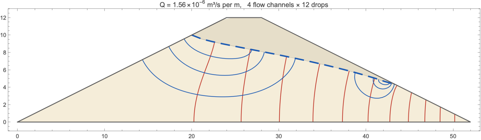
A 12 m high dam with 1V:2H slopes and a 4 m crest retains 10 m of water. The phreatic surface (dashed) and the exit point on the downstream slope are found iteratively; the seepage face below the exit point gets the h = y condition automatically:
In[145]:=
damSpec = <|"Profile" -> {{0., 0.}, {52., 0.}, {28., 12.}, {24., 12.}},
"UpstreamLevel" -> 10., "DownstreamLevel" -> 0.,
"kx" -> 1.*^-6, "ky" -> 1.*^-6|>;
damSol = SeepageUnconfined[damSpec, "Points" -> 20];
{damSol["Q"], damSol["ExitPoint"], damSol["Iterations"], damSol["Converged"]}
Out[147]=
{1.55582×
-6
10
,{43.3666,4.31669},5,True}
In[148]:=
FlowNet[damSol, "PotentialDrops" -> 12, "FlowChannels" -> 4, ImageSize -> 850]
Out[148]=

Zoned dam with a clay core

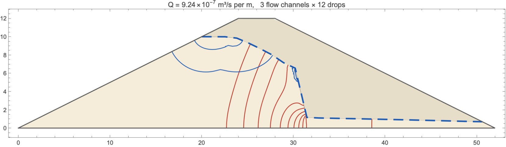
Same dam with a central low-permeability core (k = 5×10^-8 vs 10^-5 m/s shells). Layers are listed in priority order — the first polygon containing a point supplies its conductivity. Nearly all head is dissipated across the core and the phreatic surface plunges to a low level in the free-draining downstream shell.
In[149]:=
coreSpec = <|"Profile" -> {{0., 0.}, {52., 0.}, {28., 12.}, {24., 12.}},
"UpstreamLevel" -> 10., "DownstreamLevel" -> 0.,
"Layers" -> {
<|"Polygon" -> {{20., 0.}, {32., 0.}, {28., 12.}, {24., 12.}}, "kx" -> 5.*^-8, "ky" -> 5.*^-8|>,
<|"Polygon" -> {{0., 0.}, {52., 0.}, {28., 12.}, {24., 12.}}, "kx" -> 1.*^-5, "ky" -> 1.*^-5|>}|>;
coreSol = SeepageUnconfined[coreSpec, "Points" -> 24];
{coreSol["Q"], coreSol["ExitPoint"]}
Out[151]=
{9.24492×
-7
10
,{50.6071,0.696426}}
In[152]:=
FlowNet[coreSol, "PotentialDrops" -> 12, "FlowChannels" -> 3, ImageSize -> 850]
Out[152]=
TerraLapsus slope: seepage through a 1:2 slope
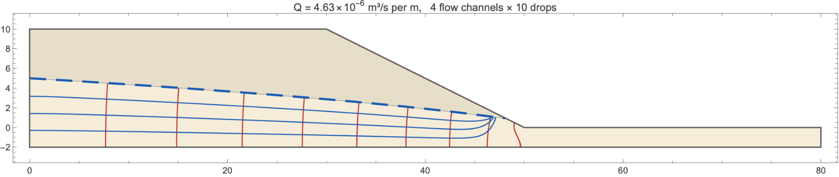
A 10 m high 1V:2H slope. The upstream water table stands 5 m above toe ground level (i.e. 5 m below the upper ground surface); downstream the water is at ground level. The impermeable model base is 2 m below the base of the slope. The datum (y = 0) is the downstream ground level at the toe. All parameters are named below; the solver finds the phreatic surface, the seepage-face exit point on the slope, and Q. For comparison, Dupuit gives Q ≈ k (hu² - hd²)/(2 Lflow) with saturated thicknesses measured from the base.
In[153]:=
Hslope = 10.; (* slope height, m *)
mSlope = 2.; (* slope 1V : mH, i.e. 1:2 *)
yToe = 0.; (* downstream (toe) ground level = datum, m *)
yTop = yToe + Hslope; (* upper ground level, m *)
yBase = yToe - 2.; (* impermeable base, 2 m below base of slope, m *)
huSlope = 5.; (* u/s water table: 5 m above toe level (5 m below upper ground), m *)
hdSlope = 0.; (* d/s water at ground level, m *)
kSlope = 1.*^-5; (* isotropic permeability, m/s *)
xCrest = 30.; (* crest position: 30 m of upper ground upstream, m *)
xToe = xCrest + mSlope Hslope; (* toe at x = 50 m *)
xEnd = 80.; (* 30 m of lower ground downstream, m *)
​
slopeProfile = {{0., yBase}, {xEnd, yBase}, {xEnd, yToe}, {xToe, yToe}, {xCrest, yTop}, {0., yTop}};
slopeSpec = <|"Profile" -> slopeProfile,
"UpstreamLevel" -> huSlope, "DownstreamLevel" -> hdSlope,
"UpstreamFace" -> {{0., yBase}, {0., yTop}},
"DownstreamFace" -> {{xEnd, yBase}, {xEnd, yToe}, {xToe, yToe}, {xCrest, yTop}},
"kx" -> kSlope, "ky" -> kSlope|>;
​
slopeSol = SeepageUnconfined[slopeSpec, "Points" -> 24];
{slopeSol["Q"], slopeSol["ExitPoint"], slopeSol["Iterations"], slopeSol["Converged"]}
Out[169]=
{4.62908×
-6
10
,{48.1019,0.949046},14,True}
In[170]:=
FlowNet[slopeSol, "PotentialDrops" -> 10, "FlowChannels" -> 4, ImageSize -> 950]
Out[170]=
The phreatic surface and pore pressures below it can be passed straight to a slope-stability analysis (e.g. TerraLapsus):
In[171]:=
slopeSol["PhreaticSurface"]
In[172]:=
slopeSol["PorePressure"][40., 0.]/1000. (* pore pressure in kPa at a point *)

Rainfall on the slope (raised water table, unsaturated zone)

Surface infiltration is added to any unconfined problem with "Rainfall" in mm/day (or "Recharge" in m/s). The rain is assumed to percolate vertically through the unsaturated zone and recharge the water table beneath, so it raises the water table and the pore pressures — the driver of most rainfall-induced slope failures. The water table is capped at the ground surface (excess is shed as runoff); the gap between them is returned as "UnsaturatedZone" and shaded in the flow net. Re-using slopeSpec from Example 3, compare dry ground with 40 mm/day of rain:
In[173]:=
slopeWet = SeepageUnconfined[slopeSpec, "Points" -> 24, "Rainfall" -> 40.];
{slopeWet["Q"], slopeWet["UnsaturatedThickness"], slopeWet["WaterTableDaylights"],
slopeWet["PorePressure"][40., 0.]/1000. - slopeSol["PorePressure"][40., 0.]/1000. (* rise in pore pressure at a point, kPa *)}
In[175]:=
FlowNet[slopeWet, "PotentialDrops" -> 10, "FlowChannels" -> 4, ImageSize -> 950]
"UnsaturatedThickness" is {min, max} of the gap between water table and ground; when the minimum falls to zero the water table daylights on the slope face ("WaterTableDaylights" -> True) and that stretch becomes a runoff/seepage face. Increase the rainfall until it daylights to find the critical intensity for the slope.

Named problems and a pore-pressure map with suction

Pass "Name" -> "id" to any solver to store its result under TerraPercolatio["id"]. Several independent problems can then coexist in one notebook and re-running one never disturbs the others — no shared state, no variable clashes. Here the dry and wet slopes are stored side by side:
In[176]:=
SeepageUnconfined[slopeSpec, "Name" -> "dry", "Points" -> 24];
SeepageUnconfined[slopeSpec, "Name" -> "wet", "Points" -> 24, "Rainfall" -> 40.];
{TerraPercolatio[],
TerraPercolatio["dry"]["Rainfall_mmday"], TerraPercolatio["wet"]["Rainfall_mmday"]}
A pore-pressure map of an unconfined solution now extends above the water table into the unsaturated zone, contouring the negative pore pressure (suction) clipped to "SuctionCap" metres of head (default 1 m ≈ 9.81 kPa) — the tension cut-off used in slope stability. Blue is positive pressure below the dashed water table, brown is suction above it:
In[179]:=
SeepagePlot[TerraPercolatio["wet"], "PorePressure", "SuctionCap" -> 1., ImageSize -> 820]

Anisotropic slope with a thin permeable drainage seam

A strongly anisotropic slope soil (kx = 1×10^-7 m/s, ky = 1×10^-9 = 0.01 kx, so flow is almost horizontal) contains a thin, highly permeable seam from y = 4 to y = 4.5 (kx = ky = 1×10^-5, 100× the bulk kx) that acts as an internal drainage layer. Layers are searched in order, so the seam polygon (listed first) takes priority inside its band and the bulk soil fills the rest. Because the unconfined multi-layer solver uses pointwise conductivities on a single mesh, a small "MeshSize" is given to resolve the 0.5 m seam.
Flow net: streamlines crowd into the seam and the equipotentials refract sharply across it — most of the discharge is carried horizontally along the seam to the toe. (Some streamline raggedness across the 0.5 m seam is the pointwise-k mesh resolving a 100–10000× contrast; refine "MeshSize" to smooth it.)
In[42]:=
FlowNet[seamSol, "PotentialDrops" -> 10, "FlowChannels" -> 5, ImageSize -> 900]
The total-head map shows the consequence for stability: above the seam the tiny ky keeps the head high (water perched, drains only slowly), while the seam concentrates the head drop and relieves the slope below it.
In[43]:=
SeepagePlot[seamSol, "Head", "IncludeSuction" -> False, Contours -> 20, ImageSize -> 900]

Slope under rainfall: pore pressures for a stability analysis (TerraLapsus)

This ties the slope work together into an output for a limit-equilibrium stability program such as TerraLapsus, using the anisotropic slope with the permeable drainage seam from Example 3d. The slope is run under steady rainfall (mm/day), which raises the water table; the pore-pressure field is then the input the stability analysis needs. PorePressureField[sol] returns u[x,y] in kPa — the FEM value below the water table and capped hydrostatic suction above it, with a tension cut-off at "SuctionCap" metres of head (default 1 m). Sampling it on a grid gives a pore-pressure field to import; the phreatic line is exported too as a piezometric surface.
Physics note: rainfall can only infiltrate as fast as the soil's vertical permeability ky allows. If the applied rainfall exceeds ky the water table mounds unrealistically (the surplus should run off), so the base soil here uses ky = 0.1 kx (1×10^-7 m/s) with rainfall 5 mm/day ≈ 5.8×10^-8 m/s < ky. With the near-impermeable ky of Example 3d, rain would simply run off.
In[44]:=
baseProfile = {{0., -2.}, {75., -2.}, {75., 0.}, {50., 0.}, {30., 10.}, {0., 10.}};
seam = <|"Polygon" -> {{-5., 4.}, {80., 4.}, {80., 4.5}, {-5., 4.5}},
"kx" -> 1.*^-5, "ky" -> 1.*^-5|>; (* permeable drainage seam *)
baseSoil = <|"Polygon" -> baseProfile, "kx" -> 1.*^-6, "ky" -> 1.*^-7|>; (* ky = 0.1 kx *)
slopeRainSol = SeepageUnconfined[<|"Profile" -> baseProfile,
"UpstreamLevel" -> 8., "DownstreamLevel" -> 0.,
"UpstreamFace" -> {{0., -2.}, {0., 10.}},
"DownstreamFace" -> {{75., -2.}, {75., 0.}, {50., 0.}, {30., 10.}},
"Layers" -> {seam, baseSoil}|>,
"Points" -> 24, "MeshSize" -> 0.15, "Rainfall" -> 5., "Name" -> "slopeRain"];
{slopeRainSol["Q"], slopeRainSol["HeadRange"], slopeRainSol["WaterTableDaylights"]}
The pore-pressure map used for the stability check: positive pressure (blue) below the dashed water table, capped suction (brown) above it. Raise "SuctionCap" to allow more suction, or set it to a tiny value for no tension.
In[49]:=
SeepagePlot[slopeRainSol, "PorePressure", "SuctionCap" -> 1., ImageSize -> 860]
Build the pore-pressure grid and the piezometric line, and write them to CSV for import into TerraLapsus (u in kPa; divide by 9.81 for pressure head in metres). Only points inside the soil body are written.
In[50]:=
u = PorePressureField[slopeRainSol, "SuctionCap" -> 1.];
grid = Flatten[Table[Module[{v = u[x, y]},
If[MissingQ[v], Nothing, {x, y, Round[v, 0.1]}]],
{x, 0., 75., 2.}, {y, -2., 10., 0.5}], 1];
Export["slope_pwp_grid.csv", Prepend[grid, {"x_m", "y_m", "u_kPa"}]];
Export["slope_phreatic.csv",
Prepend[Round[slopeRainSol["PhreaticSurface"], 0.01], {"x_m", "z_watertable_m"}]];
{Length[grid], MinMax[grid[[All, 3]]]}
Axisymmetric flow to a pumped well (drawdown cone)
Unconfined radial flow to a fully penetrating well in an aquifer on an impermeable base, solved in (r, z). SeepageWell finds the phreatic surface (cone of depression) and the seepage face on the well screen (between the pumped water level and the exit point) iteratively; the Stokes stream function from the dual problem gives flow tubes of equal discharge. Compare Q with the Dupuit-Thiem formula π k (H² - hw²)/ln(R/rw), which ignores the seepage face. All parameters are named below.
In[55]:=
rWell = 0.3; (* well radius, m *)
Rinf = 100.; (* radius of influence: far-field water table held at r = R, m *)
Haq = 20.; (* far-field water table above the impermeable base, m *)
hWell = 8.; (* pumped water level in the well, m *)
krWell = 1.*^-4; kzWell = 1.*^-4; (* radial / vertical permeability, m/s *)
​
wellSpec = <|"WellRadius" -> rWell, "OuterRadius" -> Rinf,
"FarWaterTable" -> Haq, "WellWaterLevel" -> hWell,
"kr" -> krWell, "kz" -> kzWell|>;
​
wellSol = SeepageWell[wellSpec, "Points" -> 30];
{wellSol["Q"], wellSol["DupuitQ"], wellSol["ExitPoint"], wellSol["Converged"]}
The seepage face on the screen runs from the well water level (▽, 8 m) up to the exit point (≈14.2 m). Equal head drops fall at geometrically spaced radii, as radial-flow theory requires. Axes are (r, z); the plot is zoomed to r ≤ 60 m.
In[65]:=
FlowNet[wellSol, "PotentialDrops" -> 12, "FlowChannels" -> 8,
"WaterLevels" -> {{hWell, {0., rWell}}},
PlotRange -> {{0, 60}, {0, 22}}, ImageSize -> 900]
3D flow into a rectangular excavation
A 10 m × 16 m excavation behind sheet-pile walls, dewatered to a floor 3 m below ground, in a 10 m stratum over an impermeable base. One quarter is modelled with symmetry planes at x = 0 and y = 0 (both natural no-flow boundaries). The walls and the excavated void are subtracted from the domain by constructive solid geometry, so wall faces are true no-flow boundaries. The far-field water table is held at ground level. All parameters are named below:
In[66]:=
D3 = 10.; (* stratum thickness: impermeable base z = 0, ground z = 10 *)
axq = 5.; (* excavation half-length in x (full length 10 m) *)
byq = 8.; (* excavation half-width in y (full width 16 m) *)
tw = 0.4; (* wall thickness, m *)
ztip3 = 4.; (* wall toe elevation: 6 m walls, 3 m embedment below the floor *)
zf = 7.; (* excavation floor = water level inside (dewatered), m *)
hFar = 10.; (* far-field head: water table at ground level, m *)
LxQ = 40.; LyQ = 40.; (* plan extent of the quarter model, m *)
k3 = 1.*^-5; (* isotropic permeability, m/s *)
​
wallX = Cuboid[{axq, 0., ztip3}, {axq + tw, byq + tw, D3}];
wallY = Cuboid[{0., byq, ztip3}, {axq + tw, byq + tw, D3}];
void = Cuboid[{0., 0., zf}, {axq, byq, D3}];
reg3 = RegionDifference[Cuboid[{0., 0., 0.}, {LxQ, LyQ, D3}],
RegionUnion[wallX, wallY, void]];
mesh3 = ToElementMesh[reg3, MaxCellMeasure -> 30.,
MeshRefinementFunction -> Function[{v, vol},
Module[{c = Mean[v]}, vol > If[c[[1]] < 10 && c[[2]] < 13, 0.5, 30.]]],
"MeshOrder" -> 2];
​
h3 = NDSolveValue[{Laplacian[h[x, y, z], {x, y, z}] == 0,
DirichletCondition[h[x, y, z] == hFar, x >= LxQ - 10.^-4 || y >= LyQ - 10.^-4],
DirichletCondition[h[x, y, z] == zf,
z >= zf - 10.^-4 && z <= zf + 10.^-4 && x <= axq + 10.^-4 && y <= byq + 10.^-4]},
h, {x, y, z} ∈ mesh3];
Total inflow (4 × the quarter-model flux through the floor) and exit gradients on the floor — note the 3D result that the pit corner is more critical than mid-wall:
In[83]:=
dzh = Derivative[0, 0, 1][h3]; dxh = Derivative[1, 0, 0][h3];
Qtot3 = 4. NIntegrate[k3 dzh[x, y, zf - 10.^-3], {x, 0., axq}, {y, 0., byq},
AccuracyGoal -> 4, PrecisionGoal -> 4];
{Abs[Qtot3],
Abs[dzh[axq - 0.3, 1., zf - 10.^-3]], (* exit gradient, mid long wall *)
Abs[dzh[axq - 0.3, byq - 0.3, zf - 10.^-3]], (* exit gradient, corner *)
Abs[dzh[0.1, 0.1, zf - 10.^-3]]} (* exit gradient, centre *)
Section on the symmetry plane y = 0: equipotentials (red), streamlines (blue), water levels (▽) at ground level far away and at floor level in the pit:
In[86]:=
soilY0 = Function[{x, z}, ! (axq <= x <= axq + tw && z >= ztip3) && ! (x <= axq && z >= zf)];
eqp = ContourPlot[h3[x, 0., z], {x, 0., 20.}, {z, 0., D3},
RegionFunction -> soilY0, Contours -> Range[7.25, 9.75, 0.25],
ContourShading -> None, ContourStyle -> Directive[RGBColor[0.75, 0.2, 0.15], AbsoluteThickness[1.2]],
PlotPoints -> 70];
stp = StreamPlot[{-dxh[x, 0., z], -dzh[x, 0., z]}, {x, 0., 20.}, {z, 0., D3},
RegionFunction -> soilY0, StreamPoints -> Fine, StreamColorFunction -> None,
StreamStyle -> Directive[RGBColor[0.1, 0.35, 0.7], AbsoluteThickness[1.]]];
geo = Graphics[{
{EdgeForm[{GrayLevel[0.4]}], RGBColor[0.96, 0.93, 0.85], Rectangle[{0, 0}, {20, D3}]},
{GrayLevel[0.55], Rectangle[{0, zf}, {axq, D3}]},
{GrayLevel[0.25], Rectangle[{axq, ztip3}, {axq + tw, D3}]},
{RGBColor[0.1, 0.45, 0.85], AbsoluteThickness[1.6], Line[{{0, zf}, {axq, zf}}],
Text[Style["▽", RGBColor[0.1, 0.45, 0.85], 13], {2., zf}, {0, -0.9}],
Line[{{axq + tw, D3}, {20, D3}}],
Text[Style["▽", RGBColor[0.1, 0.45, 0.85], 13], {14., D3}, {0, -0.9}]}}];
Show[geo, eqp, stp, Frame -> True, AspectRatio -> Automatic, ImageSize -> 800,
PlotLabel -> "3D excavation - section on symmetry plane y = 0"]
Plan view of the piezometric drawdown at mid-depth below the floor — rectangular near the pit, becoming circular with distance:
In[91]:=
soilPlan = Function[{x, y}, ! (x <= axq + tw && y <= byq + tw)];
Show[
ContourPlot[h3[x, y, 5.5], {x, 0., 30.}, {y, 0., 30.},
RegionFunction -> soilPlan, Contours -> Range[7.5, 9.75, 0.25],
ColorFunction -> "TemperatureMap", PlotLegends -> Automatic, PlotPoints -> 60],
Graphics[{{EdgeForm[{GrayLevel[0.25]}], GrayLevel[0.55], Rectangle[{0, 0}, {axq + tw, byq + tw}]},
Text[Style["excavation\n(quarter)", White, 11], {2.7, 4.}]}],
Frame -> True, AspectRatio -> Automatic, ImageSize -> 520,
PlotLabel -> "plan: head at z = 5.5 m"]
Parallel drainage trenches at a spacing (water-table lowering)
Design of linear drains to lower the water table (e.g. for slope stability): trenches at spacing S collect steady infiltration q. One half-cell is modelled from a drain to the mid-spacing divide, which is a no-flow symmetry boundary ("UpstreamNoFlow" -> True). Recharge crosses the phreatic surface ("Recharge" -> q), so streamlines start on the water table and the stream function ramps by the cumulative recharge. The solver finds the water-table mound; the design check is the apex height midway between drains, which the Donnan/Hooghoudt formula hmax = Sqrt[hd² + q L²/k] approximates. All parameters are named below:
In[93]:=
Sdr = 20.; (* drain spacing (centre to centre), m *)
wdr = 0.5; (* drain trench half-width, m *)
hDrain = 1.5; (* water level in the drain above the impermeable base, m *)
zGnd = 6.; (* ground level above the base, m *)
qInf = 5.*^-7;(* steady infiltration (recharge), m/s (~43 mm/day) *)
kDr = 1.*^-5; (* soil permeability, m/s *)
Ldr = Sdr/2 - wdr; (* flow length: divide to drain wall = 9.5 m *)
​
drainSpec = <|"Profile" -> {{0., 0.}, {Ldr, 0.}, {Ldr, zGnd}, {0., zGnd}},
"UpstreamLevel" -> 3., (* initial guess for the water-table apex *)
"DownstreamLevel" -> hDrain,
"UpstreamFace" -> {{0., 0.}, {0., zGnd}}, (* mid-spacing divide *)
"DownstreamFace" -> {{Ldr, 0.}, {Ldr, zGnd}}, (* drain wall *)
"kx" -> kDr, "ky" -> kDr|>;
​
drainSol = SeepageUnconfined[drainSpec, "Points" -> 24,
"Recharge" -> qInf, "UpstreamNoFlow" -> True];
{drainSol["Q"], qInf Ldr, (* outflow vs recharge balance *)
drainSol["PhreaticSurface"][[1, 2]], (* FEM water-table apex *)
Sqrt[hDrain^2 + qInf Ldr^2/kDr]} (* Donnan estimate *)
In[105]:=
FlowNet[drainSol, "PotentialDrops" -> 8, "FlowChannels" -> 8,
"WaterLevels" -> {{hDrain, {Ldr, Ldr + 2 wdr}}},
PlotRange -> {{-0.2, Ldr + 2 wdr + 0.2}, {-0.3, zGnd + 0.4}}, ImageSize -> 800]
To try a different spacing just change Sdr and re-run; the apex height is the number to check against the required water-table level.
Line of wellpoints at a spacing (excavation dewatering)
Design of a line of wellpoints (e.g. around an excavation): one well per spacing s is modelled in a 3D slab between vertical symmetry planes, y = 0 through the well and y = s/2 midway to the next well; the plane of the well line (x = 0) is no-flow, so supply comes from one side, as for a perimeter ring. The aquifer is treated as a confined slab with the initial water table as its lid (a good approximation for modest drawdown ratios). The key design outputs are the discharge per well and the residual head midway between wells — the highest water level left on the line. All parameters are named below:
In[67]:=
sWp = 3.; (* wellpoint spacing along the line, m *)
rWp = 0.25; (* effective wellpoint radius (incl. sand filter), m *)
DWp = 10.; (* saturated thickness: impermeable base z = 0, water table z = 10 *)
HWp = 10.; (* far-field head, m *)
hwWp = 3.; (* operating (suction) level in the wellpoints, m *)
zScr = 8.; (* top of screen: screened from the base to 8 m *)
LWp = 50.; (* distance to the far-field supply boundary, m *)
kWp = 1.*^-5; (* permeability, m/s *)
​
regW = RegionDifference[Cuboid[{0., 0., 0.}, {LWp, sWp/2, DWp}],
Cylinder[{{0., 0., -0.5}, {0., 0., zScr}}, rWp]];
meshW = ToElementMesh[regW, MaxCellMeasure -> 30.,
MeshRefinementFunction -> Function[{v, vol},
Module[{r = Norm[Mean[v][[1 ;; 2]]]},
vol > Which[r < 2., 0.01, r < 8., 0.5, True, 30.]]],
"MeshOrder" -> 2];
hW = NDSolveValue[{Laplacian[h[x, y, z], {x, y, z}] == 0,
DirichletCondition[h[x, y, z] == HWp, x >= LWp - 10.^-4],
DirichletCondition[h[x, y, z] == hwWp,
x^2 + y^2 <= (rWp + 0.02)^2 && z <= zScr + 10.^-3]},
h, {x, y, z} ∈ meshW];
​
dxhW = Derivative[1, 0, 0][hW]; dzhW = Derivative[0, 0, 1][hW];
QperWell = 2. Abs[NIntegrate[kWp dxhW[LWp - 10.^-3, y, z],
{y, 0., sWp/2}, {z, 0., DWp}, AccuracyGoal -> 4, PrecisionGoal -> 4]];
{QperWell, (* discharge per wellpoint, m³/s *)
hW[0.011, sWp/2, DWp - 10.^-3], (* residual head midway between wells *)
hW[0.011, sWp/2, 5.]} (* ditto at mid-screen depth *)
Section through a well: flow converges vertically onto the screen (the top 2 m are unscreened), which is why the residual head midway is governed by partial penetration rather than plan spacing here. Water levels (▽): undisturbed table at 10 m, suction level 3 m in the well:
In[83]:=
Show[
Graphics[{{EdgeForm[{GrayLevel[0.4]}], RGBColor[0.96, 0.93, 0.85], Rectangle[{0, 0}, {15, DWp}]},
{GrayLevel[0.25], Rectangle[{0, 0}, {rWp, zScr}]},
{RGBColor[0.1, 0.45, 0.85], AbsoluteThickness[1.6], Line[{{rWp, hwWp}, {1.2, hwWp}}],
Text[Style["▽", RGBColor[0.1, 0.45, 0.85], 12], {0.75, hwWp}, {0, -0.9}],
Line[{{rWp, DWp}, {15, DWp}}],
Text[Style["▽", RGBColor[0.1, 0.45, 0.85], 12], {10., DWp}, {0, -0.9}]}}],
ContourPlot[hW[x, 0., z], {x, rWp, 15.}, {z, 0., DWp},
Contours -> Range[3.5, 9.5, 0.5], ContourShading -> None,
ContourStyle -> Directive[RGBColor[0.75, 0.2, 0.15], AbsoluteThickness[1.2]], PlotPoints -> 60],
StreamPlot[{-dxhW[x, 0., z], -dzhW[x, 0., z]}, {x, rWp, 15.}, {z, 0., DWp},
StreamPoints -> Fine, StreamColorFunction -> None,
StreamStyle -> Directive[RGBColor[0.1, 0.35, 0.7], AbsoluteThickness[1.]]],
Frame -> True, AspectRatio -> Automatic, ImageSize -> 800,
PlotLabel -> "wellpoint line - section through a well (y = 0)"]
Plan view of the water table near the line (mirrored across the symmetry planes to show two spacings). The contour scallops between wells die out within about half a spacing; the midway residual head is the design value to compare with the required drawdown. Increase sWp and re-run to see the scallops deepen:
In[84]:=
Show[
ContourPlot[hW[x, sWp/2 - Abs[Mod[y, sWp] - sWp/2], DWp - 10.^-3],
{x, 0.01, 5.}, {y, 0., 2 sWp},
Contours -> Range[3.1, 4.7, 0.1], ColorFunction -> "TemperatureMap",
PlotLegends -> Automatic, PlotPoints -> 90, Exclusions -> None,
RegionFunction -> Function[{x, y}, x^2 + Min[Mod[y, sWp], sWp - Mod[y, sWp]]^2 > (rWp + 0.01)^2]],
Graphics[{GrayLevel[0.2], Disk[{0, 0}, rWp], Disk[{0, sWp}, rWp], Disk[{0, 2 sWp}, rWp],
Text[Style["wells", 11], {0.55, 4.4}]}],
Frame -> True, AspectRatio -> Automatic, ImageSize -> 560,
PlotLabel -> "plan: water table near the wellpoint line (z = 10 m)"]
Working with the solution object
Every solver returns an Association. Useful keys: "Head" (interpolating function h[x,y]), "Psi" (stream function), "Q" (discharge per metre), "Velocity" and "Gradient" (functions of x,y), "PorePressure" (Pa), "Mesh", and for unconfined problems "PhreaticSurface" and "ExitPoint". BoundaryFlux integrates outward flux over any boundary you select with a predicate:

© 2026 Wolfram. All rights reserved.

  • Legal & Privacy Policy
  • Contact Us
  • WolframAlpha.com
  • WolframCloud.com