Genomic comparisons (2)
Some viral genomes in the FASTA database:
A list of corresponding genome identifiers in FASTA format:
Import these using the resource function ImportFASTA; this takes a bit of time:
Get the genomic sequence strings:
Create vectors for these sequences:
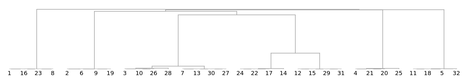
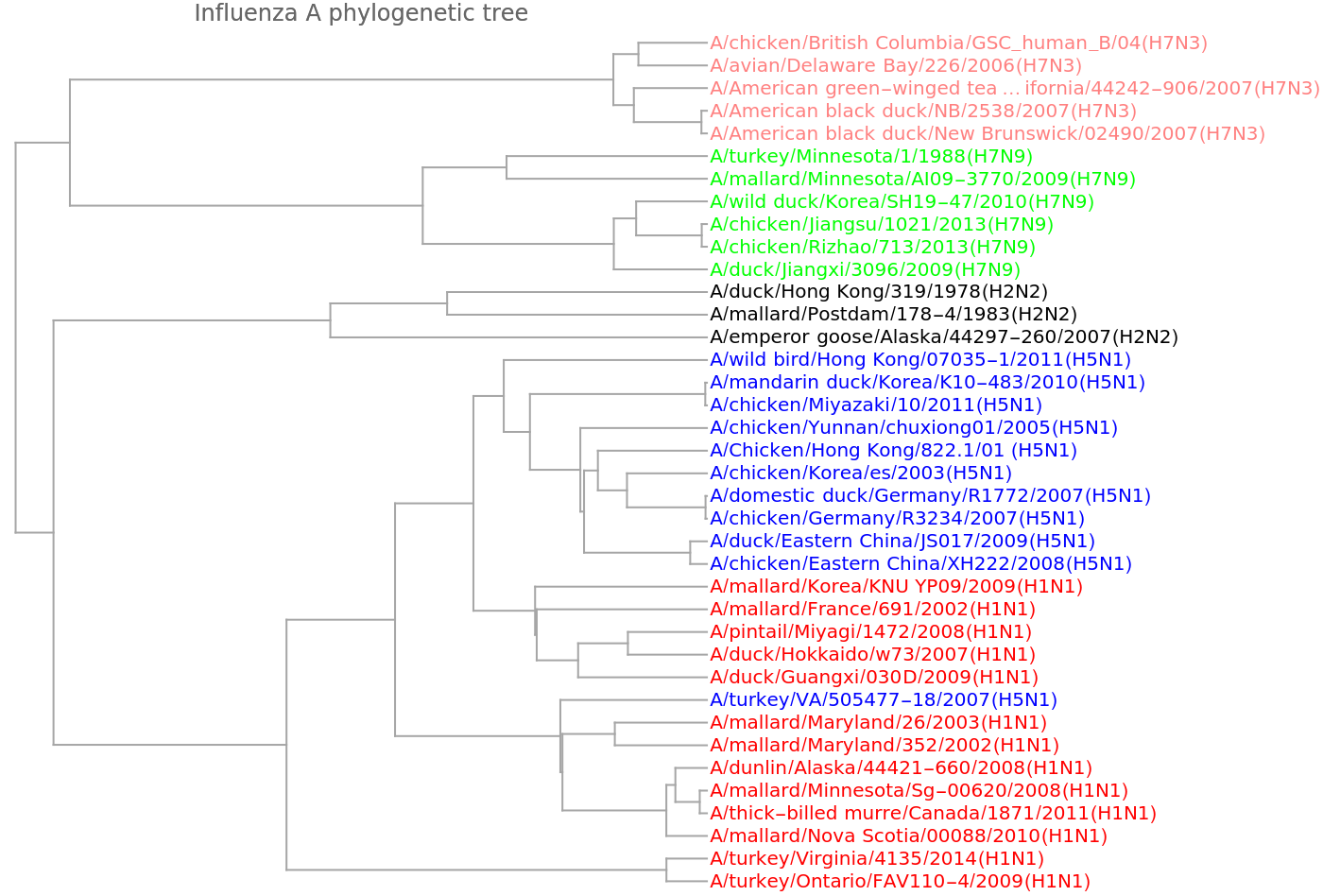
Show a dendrogram using different colors for the distinct viral types:
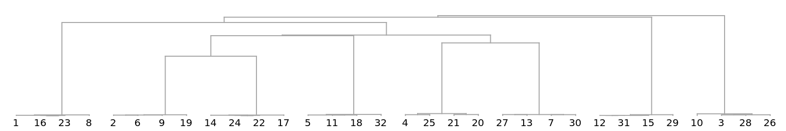
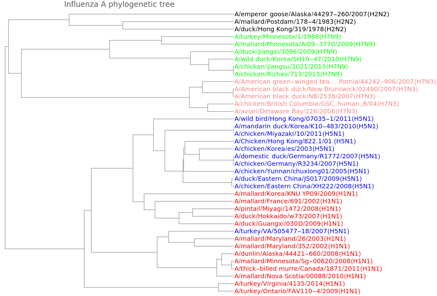
We get a similar dendrogram from the "GenomeFCGR" method:
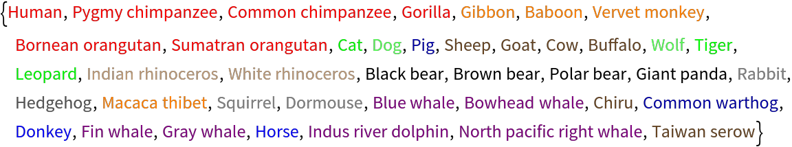
We use a standard test set of mammal species:
Import the sequences from the FASTA site:
Form vectors from these genome strings:
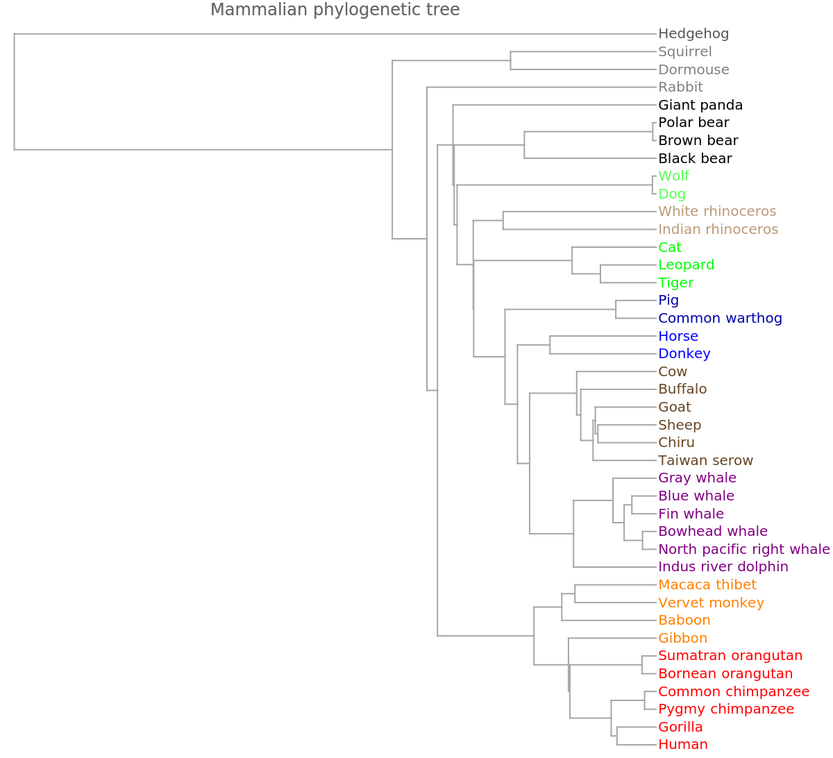
Set up data for a phylogenetic tree:
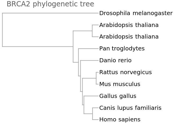
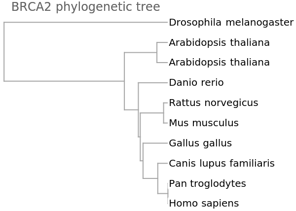
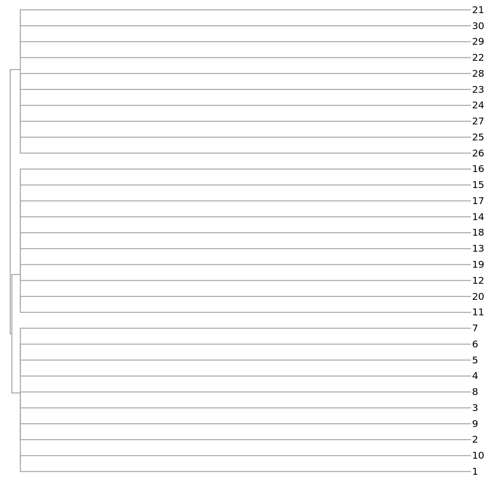
Show the dendrogram obtained from this encoding of the genomes into vectors:
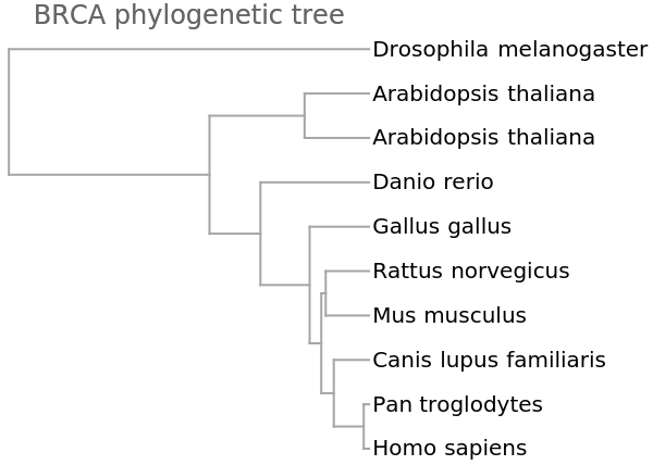
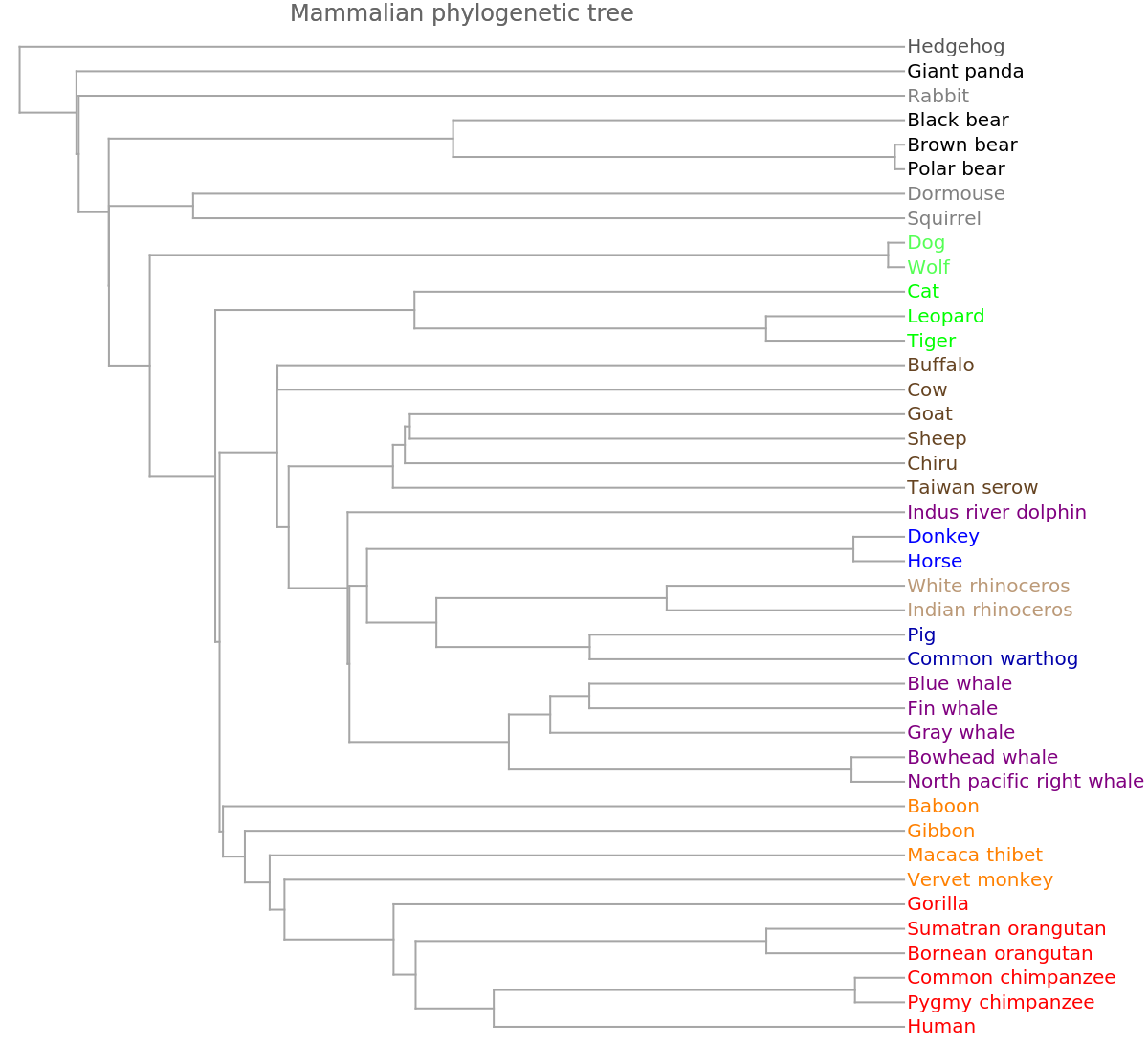
The genome FCGR encoding gives a similar grouping:
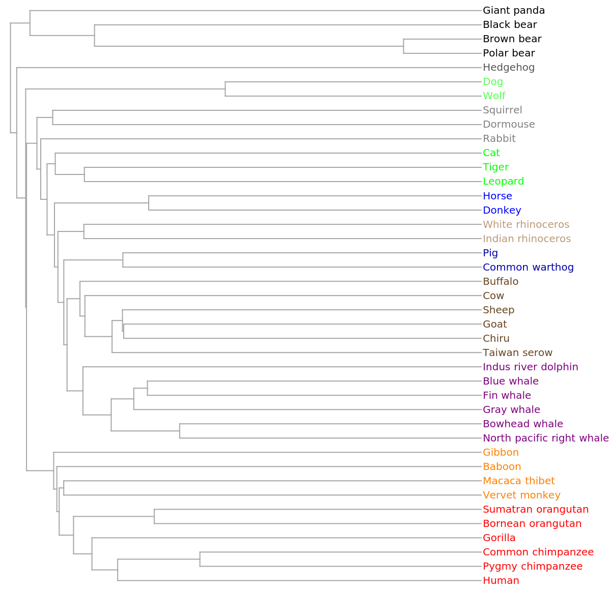
Compare to the resource function PhylogeneticTreePlot:
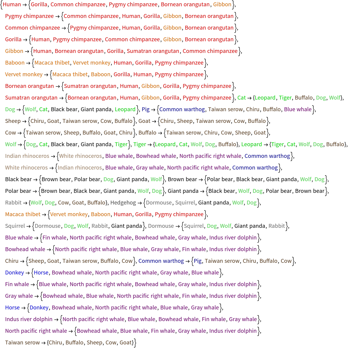
Find five nearest neighbors for each species:
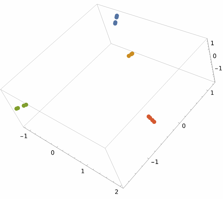
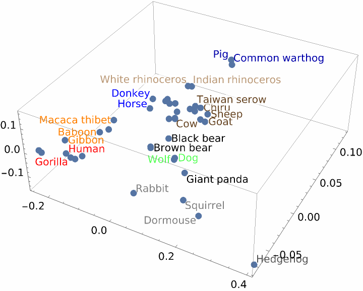
Use the resource function MultidimensionalScaling to reduce to three dimensions for visualization:
Authorship identification (3)
We can use string vectors for determining when substrings might have a similar source.
Obtain several English texts from ExampleData:
Split into sets of substrings of length 2000:
Create vectors of length 80 for these strings:
Split into odd and even numbered substrings for purposes of training and testing a classifier:
Train a neural net to classify the different texts:
Check that 99% of the test strings are classified correctly:
Authorship of nineteenth century French novels. Data is from the reference Understanding and explaining Delta measures for authorship attribution.The importing step can take as much as a few minutes.
Import 75 French novels with three by each of 25 authors, clipping the size of the larger ones in order to work with strings of comparable lengths:
Partition each into substrings of 10000 characters and split into training (two novels per author) and test (one per author) sets:
Create vectors of length 200:
A simple classifier associates around 80% of the substrings in the test set with the correct author:
A simple neural net associates nearly 90% with the actual author:
We apply string vector similarity to the task of authorship attribution. We use as an example the Federalist Papers, where authorship of several was disputed for around 175 years. The individual authors were Alexander Hamilton, James Madison and John Jay. Due to happenstance of history (Hamilton may have recorded his claims of authorship in haste, with his duel with Aaron Burr encroaching), twelve were claimed by both Hamilton and Madison. The question was largely settled in the 1960's (see Author Notes). Nevertheless this is generally acknowledged as a difficult test for authorship attribution methods. We use some analysis of n-gram strings to show one method of analysis.
Import data, split into individual essays and remove author names and boilerplate common to most or all articles:
Separate out the three essays jointly attributed to Hamilton and Madison, as well as the five written by John Jay, and show the numbering for the disputed set:
We split each essay into substrings of length 2000 and create vectors of length 80, using a larger-than-default setting for the number of n-grams to consider:
Remove from consideration several essays of known authorship, as well as the last chunk from each remaining essay of known authorship; these provide two validation sets for which we will assess the quality of the classifier:
Since Hamilton wrote far more essays than Madison, we removed far more of his from the training set and now check that the contributions of the two authors to the training set are not terribly different in size (that is, within a factor of 1.5):
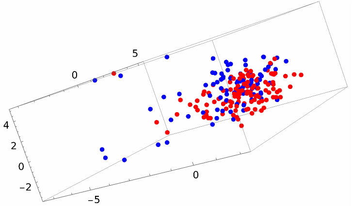
The two sets reduced to three dimensions, with red dots for Hamilton's strings and blue dots for Madison's, do not appear to separate nicely:
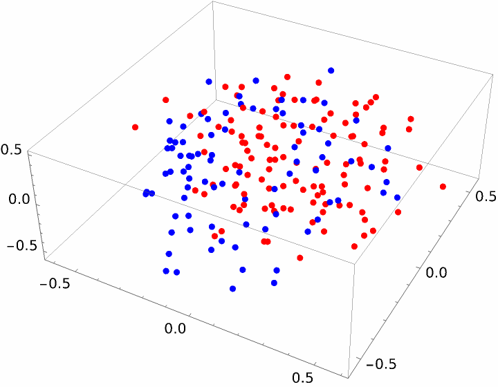
A different method gives a result that looks better but still does not show an obvious linear space separation:
Using nearest neighbors (as done for the genome set examples) of these vectors to classify authorship is prone to failure, so instead we train a neural net, with numeric outcomes of 1 for Hamilton authorship and 2 for Madison:
Now assess correctness percentage on the first validation set (withheld essays), as well as possible bias in incorrectness:
Do likewise for the second validation set (chunks withheld from the training group essays):
Both exceed 90% correct, and both show around a 10% inclination in each incorrect direction (that is, Hamilton authorship assessed as Madison or vice versa).
Assess authorship on the substrings in the test set (from the twelve disputed essays):
Tally these:
We redo this experiment, this time using the "TextFGCR" method for conversion to numeric vectors:
Repeat processing through creating a neural net classifier:
Repeat the first validation check:
Repeat the second validation check:
Both are just under 90%, and we observe this time there is a one-in-three (5/15) tendency in the first set to mistake actual Madison essays (where the first value is 2) as Hamilton's.
Again assess authorship on the substrings in the test set (from the twelve disputed essays):
And tally these:
These results are consistent with the consensus opinion supporting Madison authorship, or at least primary authorship, on the twelve disputed essays.


![createStringTable[len_Integer, strsize_Integer, changeprop_, clen_Integer, ccount_Integer] := Module[{intchars, atoz, initstr, str, newstr, stringtable, elem, rnd,
rndposns, rndsubstrings, rpos}, atoz = Flatten[{ToCharacterCode["a"], ToCharacterCode["z"]}]; intchars = RandomInteger[atoz, strsize]; initstr = StringJoin[FromCharacterCode[intchars]]; str = initstr; rnd = RandomChoice[{changeprop, 1 - changeprop} -> {True, False}, len]; stringtable = Table[If[rnd[[j]], rndposns = RandomSample[Range[strsize - clen + 1], ccount]; intchars = RandomInteger[atoz, {ccount, clen}]; rndsubstrings = (StringJoin[FromCharacterCode[#1]] &) /@ intchars; newstr = str; Do[rpos = rndposns[[k]]; newstr = StringReplacePart[newstr, rndsubstrings[[k]], {rpos, rpos + clen - 1}];, {k, ccount}]; str = newstr;]; str, {j, len}]]](https://www.wolframcloud.com/obj/resourcesystem/images/e44/e446d97f-8bde-4059-a8ff-71e60a416cd7/015d4bbe991731b8.png)
![SeedRandom[1234];
strs = RandomSample[
Flatten[Table[
createStringTable[4, 500 + Round[30*RandomReal[{-1, 1}]], .99, 2,
3], {8}]]];](https://www.wolframcloud.com/obj/resourcesystem/images/e44/e446d97f-8bde-4059-a8ff-71e60a416cd7/4420ed17ddf2e429.png)
![createStringTable[len_Integer, strsize_Integer, changeprop_, clen_Integer, ccount_Integer] := Module[{intchars, atoz, initstr, str, newstr, stringtable, elem, rnd, rndposns, rndsubstrings, rpos}, atoz = Flatten[{
ToCharacterCode["a"],
ToCharacterCode["z"]}]; intchars = RandomInteger[
atoz, strsize]; initstr = StringJoin[
FromCharacterCode[
intchars]]; str = initstr; rnd = RandomChoice[{changeprop, 1 - changeprop} -> {True, False}, len]; stringtable = Table[
If[
Part[rnd, j], rndposns = RandomSample[
Range[strsize - clen + 1], ccount]; intchars = RandomInteger[
atoz, {ccount, clen}]; rndsubstrings = Map[StringJoin[
FromCharacterCode[#]]& , intchars]; newstr = str; Do[
rpos = Part[rndposns, k]; newstr = StringReplacePart[newstr,
Part[rndsubstrings, k], {rpos, rpos + clen - 1}]; Null, {k, ccount}]; str = newstr; Null]; str, {j, len}]]
Short[strs = RandomSample[
Join[createStringTable[40, 400, .99, 2, 3], createStringTable[40, 300, .99, 2, 3], createStringTable[40, 500, .99, 2, 3]]]]](https://www.wolframcloud.com/obj/resourcesystem/images/e44/e446d97f-8bde-4059-a8ff-71e60a416cd7/7ca56f7d60055bfc.png)
![svecs1 = ResourceFunction["StringsToVectors"][strs, 3];
Short[svecs2 = Map[#/Norm[#] &, ResourceFunction["StringsToVectors"][strs, 3, "DimensionReductionMethod" -> (DimensionReduce[#, 3, Method -> "LatentSemanticAnalysis"] &)]]]](https://www.wolframcloud.com/obj/resourcesystem/images/e44/e446d97f-8bde-4059-a8ff-71e60a416cd7/123e31e8307e50e3.png)
![brca2 = SemanticInterpretation["brca2 gene", AmbiguityFunction -> All];
bcGenes = brca2[[1]];
refseqs = Through[bcGenes["ReferenceSequence"]];
species = Through[bcGenes["Species"]]](https://www.wolframcloud.com/obj/resourcesystem/images/e44/e446d97f-8bde-4059-a8ff-71e60a416cd7/6f31692ca1b1dbdd.png)
![vecs = ResourceFunction["StringsToVectors"][refseqs];
dd = Dendrogram[vecs -> species, Left, AspectRatio -> 1.1, ImageSize -> 300, PlotLabel -> "BRCA2 phylogenetic tree", DistanceFunction -> CosineDistance]](https://www.wolframcloud.com/obj/resourcesystem/images/e44/e446d97f-8bde-4059-a8ff-71e60a416cd7/547e985d858cd548.png)
![vecsNoN = ResourceFunction["StringsToVectors"][refseqsNoN];
dd = Dendrogram[vecsNoN -> species, Left, AspectRatio -> 1.1, ImageSize -> 300, PlotLabel -> "BRCA2 phylogenetic tree", DistanceFunction -> CosineDistance]](https://www.wolframcloud.com/obj/resourcesystem/images/e44/e446d97f-8bde-4059-a8ff-71e60a416cd7/748e9d6f5c4512da.png)
![vecsG = ResourceFunction["StringsToVectors"][refseqs, Method -> "GenomeFCGR"];
Dendrogram[vecsG -> species, Left, AspectRatio -> 1.1, ImageSize -> 300, PlotLabel -> "BRCA phylogenetic tree", DistanceFunction -> CosineDistance]](https://www.wolframcloud.com/obj/resourcesystem/images/e44/e446d97f-8bde-4059-a8ff-71e60a416cd7/404ad7ac5a8bc554.png)
![createStringTable[len_Integer, strsize_Integer, changeprop_, clen_Integer, ccount_Integer] := Module[{intchars, atoz, initstr, str, newstr, stringtable, elem, rnd, rndposns, rndsubstrings, rpos}, atoz = Flatten[{
ToCharacterCode["a"],
ToCharacterCode["z"]}]; intchars = RandomInteger[
atoz, strsize]; initstr = StringJoin[
FromCharacterCode[
intchars]]; str = initstr; rnd = RandomChoice[{changeprop, 1 - changeprop} -> {True, False}, len]; stringtable = Table[
If[
Part[rnd, j], rndposns = RandomSample[
Range[strsize - clen + 1], ccount]; intchars = RandomInteger[
atoz, {ccount, clen}]; rndsubstrings = Map[StringJoin[
FromCharacterCode[#]]& , intchars]; newstr = str; Do[
rpos = Part[rndposns, k]; newstr = StringReplacePart[newstr,
Part[rndsubstrings, k], {rpos, rpos + clen - 1}]; Null, {k, ccount}]; str = newstr; Null]; str, {j, len}]]
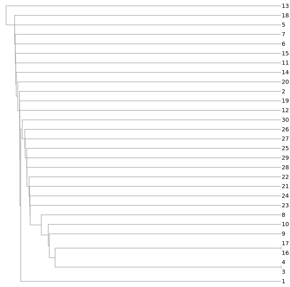
Short[strs = Join[createStringTable[10, 400, .99, 2, 3], createStringTable[10, 300, .99, 2, 3], createStringTable[10, 500, .99, 2, 3]]]](https://www.wolframcloud.com/obj/resourcesystem/images/e44/e446d97f-8bde-4059-a8ff-71e60a416cd7/5085fbc840608eb4.png)
![Dendrogram[
ResourceFunction["StringsToVectors"][strs] -> Range[Length[strs]], Left, ImageSize -> 500, AspectRatio -> 1]](https://www.wolframcloud.com/obj/resourcesystem/images/e44/e446d97f-8bde-4059-a8ff-71e60a416cd7/2e9ba367fb24440d.png)
![Dendrogram[
ResourceFunction["StringsToVectors"][strs, Method -> "GenomeFCGR"] ->
Range[Length[strs]], Left, ImageSize -> 500, AspectRatio -> 1]](https://www.wolframcloud.com/obj/resourcesystem/images/e44/e446d97f-8bde-4059-a8ff-71e60a416cd7/5e6497d111e3cbe2.png)
![stringColor[str_String] := Which[
StringContainsQ[str, "H1N1"], Red,
StringContainsQ[str, "H5N1"], Blue,
StringContainsQ[str, "H7N3"], Pink,
StringContainsQ[str, "H7N9"], Green,
StringContainsQ[str, "H2N2"], Black]
speciesViralColored = Map[Style[#, stringColor[#]] &, speciesViral];
Dendrogram[vecs -> speciesViralColored, Left, AspectRatio -> 1.2, ImageSize -> 700, PlotLabel -> "Influenza A phylogenetic tree", DistanceFunction -> CosineDistance]](https://www.wolframcloud.com/obj/resourcesystem/images/e44/e446d97f-8bde-4059-a8ff-71e60a416cd7/185802660a7a7da0.png)
![vecsG = ResourceFunction["StringsToVectors"][sequencesViral, Method -> "GenomeFCGR"];
Dendrogram[vecsG -> speciesViralColored, Left, AspectRatio -> 1.2, ImageSize -> 700, PlotLabel -> "Influenza A phylogenetic tree", DistanceFunction -> CosineDistance]](https://www.wolframcloud.com/obj/resourcesystem/images/e44/e446d97f-8bde-4059-a8ff-71e60a416cd7/3e2f4940fc7aa4f6.png)
![speciesMammal = {"Human", "Pygmy chimpanzee", "Common chimpanzee", "Gorilla", "Gibbon", "Baboon", "Vervet monkey", "Bornean orangutan", "Sumatran orangutan", "Cat", "Dog", "Pig", "Sheep", "Goat", "Cow", "Buffalo", "Wolf", "Tiger", "Leopard", "Indian rhinoceros", "White rhinoceros", "Black bear", "Brown bear", "Polar bear", "Giant panda", "Rabbit", "Hedgehog", "Macaca thibet", "Squirrel", "Dormouse", "Blue whale", "Bowhead whale", "Chiru", "Common warthog", "Donkey", "Fin whale", "Gray whale", "Horse", "Indus river dolphin", "North pacific right whale", "Taiwan serow"};
stringColor[str_String] := Which[
StringContainsQ[str, {"Human", "chimpanzee", "Gorilla", "orangutan"}],
Red,
StringContainsQ[str, {"Gibbon", "Baboon", "monkey", "thibet"}], Orange,
StringContainsQ[str, {"Tiger", "Leopard", "Cat"}], Green,
StringContainsQ[str, {"Dog", "Wolf"}],
Lighter[Green],
StringContainsQ[
str, {"Cow", "Buffalo", "Goat", "Sheep", "Chiru", "serow"}],
Darker[Brown],
StringContainsQ[str, "rhino"],
Lighter[Brown],
StringContainsQ[str, {"bear", "panda"}], Black,
StringContainsQ[str, {"mouse", "Squirrel", "Rabbit"}], Gray,
StringContainsQ[str, {"Pig", "warthog"}],
Darker[Blue],
StringContainsQ[str, {"Donkey", "Horse"}], Blue,
StringContainsQ[str, {"whale", "dolphin"}], Purple,
StringContainsQ[str, "Hedgehog"],
Darker[Gray]]
speciesMammalColored = Map[Style[#, stringColor[#]] &, speciesMammal]](https://www.wolframcloud.com/obj/resourcesystem/images/e44/e446d97f-8bde-4059-a8ff-71e60a416cd7/2ae12122e7c3ab64.png)
![Dendrogram[ngramvecs -> speciesMammalColored, Left, AspectRatio -> 1.1, ImageSize -> 600, PlotLabel -> "Mammalian phylogenetic tree", DistanceFunction -> CosineDistance]](https://www.wolframcloud.com/obj/resourcesystem/images/e44/e446d97f-8bde-4059-a8ff-71e60a416cd7/607db71be041ec18.png)
![fcgrvecs = ResourceFunction["StringsToVectors"][sequencesMammal, Method -> "GenomeFCGR"];
Dendrogram[fcgrvecs -> speciesMammalColored, Left, AspectRatio -> 1.1,
ImageSize -> 600, PlotLabel -> "Mammalian phylogenetic tree", DistanceFunction -> CosineDistance]](https://www.wolframcloud.com/obj/resourcesystem/images/e44/e446d97f-8bde-4059-a8ff-71e60a416cd7/64cba765f37b5408.png)
![ListPointPlot3D[
MapApply[Labeled, Transpose[{ResourceFunction["MultidimensionalScaling"][ngramvecs, 3], speciesMammalColored}]]]](https://www.wolframcloud.com/obj/resourcesystem/images/e44/e446d97f-8bde-4059-a8ff-71e60a416cd7/38fead4ddffc0b72.png)
![textnames = {"AeneidEnglish", "AliceInWonderland", "BeowulfModern", "CodeOfHammurabiEnglish", "DonQuixoteIEnglish", "FaustI", "GenesisKJV", "Hamlet", "OnTheNatureOfThingsEnglish", "OriginOfSpecies", "PlatoMenoEnglish", "PrideAndPrejudice", "ShakespearesSonnets"};
texts = Map[ExampleData[{"Text", #}] &, textnames];
tlen = Length[textnames];](https://www.wolframcloud.com/obj/resourcesystem/images/e44/e446d97f-8bde-4059-a8ff-71e60a416cd7/7b9bb336a9ab0bb4.png)
![substrs = Map[StringPartition[#, 2000] &, texts];
slens = Map[Length, substrs];
sposns = Map[{1, 0} + # &, Partition[Join[{0}, Accumulate[slens]], 2, 1]];](https://www.wolframcloud.com/obj/resourcesystem/images/e44/e446d97f-8bde-4059-a8ff-71e60a416cd7/2e5d25fda20b5fa1.png)
![vecsize = 80;
Timing[textVectors0 = ResourceFunction["StringsToVectors"][Flatten@substrs, vecsize];]
textVectors = Map[textVectors0[[Apply[Span, #]]] &, sposns];](https://www.wolframcloud.com/obj/resourcesystem/images/e44/e446d97f-8bde-4059-a8ff-71e60a416cd7/0b03b75d57664b99.png)
![trainVectors = textVectors[[All, 1 ;; -1 ;; 2]];
testVectors = textVectors[[All, 2 ;; -1 ;; 2]];
labeledTrain = Flatten[MapIndexed[#1 -> #2[[1]] &, trainVectors, {2}]];
labeledTest = Flatten[MapIndexed[{#1, #2[[1]]} &, testVectors, {2}], 1];](https://www.wolframcloud.com/obj/resourcesystem/images/e44/e446d97f-8bde-4059-a8ff-71e60a416cd7/5ca8b7feb412d226.png)
![net = NetChain[{1000, Tanh, tlen, Tanh, SoftmaxLayer[]}, "Input" -> vecsize, "Output" -> NetDecoder[{"Class", Range[tlen]}]]; trained = NetTrain[net, RandomSample@labeledTrain, MaxTrainingRounds -> 500];](https://www.wolframcloud.com/obj/resourcesystem/images/e44/e446d97f-8bde-4059-a8ff-71e60a416cd7/051d220b54f58c7b.png)
![results = Map[{#[[2]], trained[#[[1]]]} &, labeledTest];
tallied = Tally[results];
{tallied, N[Total[Cases[tallied, {{a_, a_}, n_} :> n]]]/Length[labeledTest]}](https://www.wolframcloud.com/obj/resourcesystem/images/e44/e446d97f-8bde-4059-a8ff-71e60a416cd7/26bfbe261dd4d944.png)

![lynxF0 = Import[
"https://github.com/cophi-wue/refcor/tree/master/French"];
lynxF1 = StringDelete[lynxF0, ":" | "\""];
lynxF2 = StringSplit[lynxF1, "tree"][[2]];
lynxF3 = StringSplit[lynxF2, "items"][[2]];
lynxF4 = StringSplit[lynxF3, "name" | "path"][[2 ;; -1 ;; 2]];
lynxF5 = Map[StringReplace[#, "," -> ""] &, lynxF4];
textlinksF = Map[StringJoin[{"https://raw.githubusercontent.com/cophi-wue/refcor/master/French/", #}] &, lynxF5];
AbsoluteTiming[novelStringsF = Table[
str0 = Import[textlinksF[[j]]];
str1 = StringTake[str0, UpTo[400000]];
str = StringDrop[StringDrop[str1, 5000], -2000],
{j, Length[lynxF5]}];]](https://www.wolframcloud.com/obj/resourcesystem/images/e44/e446d97f-8bde-4059-a8ff-71e60a416cd7/72b56c63bbf487f7.png)
![sublen = 10000;
allTrainWritings0 = Riffle[novelStringsF[[2 ;; -1 ;; 3]], novelStringsF[[3 ;; -1 ;; 3]]];
allTestWritings0 = novelStringsF[[1 ;; -1 ;; 3]];
allTrainWritings1 = Map[StringPartition[#, sublen] &, allTrainWritings0];
allTestWritings1 = Map[StringPartition[#, sublen] &, allTestWritings0];
trainlens = Map[Total, Partition[Map[Length, allTrainWritings1], 2]];
testlens = Map[Length, allTestWritings1];
allTrainWritings = Flatten[allTrainWritings1];
allTestWritings = Flatten[allTestWritings1];
trainlabels = Flatten@MapIndexed[ConstantArray[#2[[1]], #1] &, trainlens];
testlabels = Flatten@MapIndexed[ConstantArray[#2[[1]], #1] &, testlens];](https://www.wolframcloud.com/obj/resourcesystem/images/e44/e446d97f-8bde-4059-a8ff-71e60a416cd7/1d2fb5d91283dc24.png)
![vlen = 200;
AbsoluteTiming[
vecs = ResourceFunction["StringsToVectors"][
Join[allTrainWritings, allTestWritings], vlen];]
{trainvecs, testvecs} = TakeDrop[vecs, Length[allTrainWritings]];](https://www.wolframcloud.com/obj/resourcesystem/images/e44/e446d97f-8bde-4059-a8ff-71e60a416cd7/5275071460711191.png)
![cfunc = Classify[RandomSample[Thread[trainvecs -> trainlabels]], Method -> {"LogisticRegression", "OptimizationMethod" -> "LBFGS"}, "FeatureExtractor" -> None, PerformanceGoal -> "Quality"];
res = Transpose[{testlabels, cfunc[testvecs]}];
Length[Cases[res, {a_, a_}]]/N[Length[res]]](https://www.wolframcloud.com/obj/resourcesystem/images/e44/e446d97f-8bde-4059-a8ff-71e60a416cd7/00eefaa0603330f2.png)
![numauthors = Length[testlens];
trainset = RandomSample[Thread[trainvecs -> trainlabels]]; net = NetChain[{500, Ramp, Tanh, numauthors, Tanh, SoftmaxLayer[]}, "Input" -> Length[trainvecs[[1]]], "Output" -> NetDecoder[{"Class", Range[numauthors]}]]; trained = NetTrain[net, trainset, MaxTrainingRounds -> 200, RandomSeeding -> Automatic, Method -> {"ADAM", "Beta1" -> .9}];
results = Transpose[{testlabels, Map[trained, testvecs]}];
Length[Cases[results, {a_, a_}]]/N[Length[res]]](https://www.wolframcloud.com/obj/resourcesystem/images/e44/e446d97f-8bde-4059-a8ff-71e60a416cd7/03b09bc1e6069f54.png)
![fedpap = Import["https://www.gutenberg.org/files/18/18-0.txt", "Text"];
fedpap2 = StringDrop[fedpap, 1 ;; 7780];
fedpap3 = StringSplit[fedpap2, "FEDERALIST"][[2 ;; -2]];
fedpap4 = Delete[fedpap3, 71];
fedpap4[[-1]] = StringDrop[fedpap4[[-1]], -170 ;; -1];
fedpap5 = Map[StringReplace[#, "JAY" | "MADISON" | "HAMILTON" | "PUBLIUS" -> ""] &, fedpap4];
fedpap6 = Map[StringReplace[#, "From the New York Packet." | "To the People of the State of New York:" | "No." | "For the Independent Journal." -> ""] &, fedpap5];](https://www.wolframcloud.com/obj/resourcesystem/images/e44/e446d97f-8bde-4059-a8ff-71e60a416cd7/7a2b3ebcd0c79817.png)
![rng = Range[Length[fedpap4]];
authorHandM = Map[StringCases[#, "HAMILTON" ~~ Whitespace ~~ "AND" ~~ Whitespace ~~ "MADISON"] &, fedpap4];
authorHandMPosns = Complement[rng, Flatten[Position[authorHandM, {}, {1}]]];
authorHorM = Map[StringCases[#, "HAMILTON" ~~ Whitespace ~~ "OR" ~~ Whitespace ~~ "MADISON"] &, fedpap4];
authorHorMPosns = Union[{58}, Complement[rng, Flatten[Join[{58}, Position[authorHorM, {}, {1}]]]]]
authorH = Map[StringCases[#, "HAMILTON"] &, fedpap4];
authorHPosns = Complement[rng, Join[Flatten[Position[authorH, {}, {1}]], authorHorMPosns, authorHandMPosns]];
authorM = Map[StringCases[#, "MADISON"] &, fedpap4];
authorMPosns = Complement[rng, Join[Flatten[Position[authorM, {}, {1}]], authorHorMPosns, authorHandMPosns]];
authorJ = Map[StringCases[#, "JAY"] &, fedpap4];
authorJPosns = Complement[rng, Flatten[Position[authorJ, {}, {1}]]];
valRule = Flatten[Map[Thread, MapThread[
Rule, {{authorHandMPosns, authorHorMPosns, authorHPosns, authorMPosns, authorJPosns}, {"HandM", "HorM", "H", "M", "J"}}]]];
authorValues = rng /. valRule /. {"H" -> 1, "M" -> 2};](https://www.wolframcloud.com/obj/resourcesystem/images/e44/e446d97f-8bde-4059-a8ff-71e60a416cd7/0f58c992e0580c75.png)
![strsize = 2000;
substrings = Map[StringPartition[#, strsize] &, fedpap6];
slens = Map[Length, substrings];
vecsize = 80;
Timing[textVectors0 = ResourceFunction["StringsToVectors"][Flatten@substrings, vecsize, Method -> {"NGrams", "RetainCount" -> 4000}];]
sposns = Map[{1, 0} + # &, Partition[Join[{0}, Accumulate[slens]], 2, 1]];
textVectors = Map[textVectors0[[Apply[Span, #]]] &, sposns];](https://www.wolframcloud.com/obj/resourcesystem/images/e44/e446d97f-8bde-4059-a8ff-71e60a416cd7/22cea4d9777206f1.png)
![noHorMlist = Delete[rng, Map[List, authorHorMPosns, {1}]];
trainingSet = Complement[noHorMlist,
Join[authorMPosns[[1 ;; -1 ;; 10]], authorHPosns[[1 ;; -1 ;; 2]], authorJPosns, authorHandMPosns]];
trainingSetLabels = authorValues[[trainingSet]];
trainingVectors = Map[#[[1 ;; -2]] &, textVectors[[trainingSet]]];
testSet = authorHorMPosns;
testSetLabels = authorValues[[testSet]];
testSetVectors = textVectors[[testSet]];
validationSet1 = Complement[rng, Join[testSet, trainingSet, authorJPosns, authorHandMPosns]];
validationSet1Labels = authorValues[[validationSet1]];
validationSet1Vectors = textVectors[[validationSet1]];
validationSet2 = trainingSet;
validationSet2Labels = authorValues[[validationSet2]];
validationSet2Vectors = Map[#[[-1 ;; -1]] &, textVectors[[validationSet2]]];
alltrainingVectors = Apply[Join, trainingVectors];
alltrainingLabels = Flatten[Table[
ConstantArray[trainingSetLabels[[j]], Length[trainingVectors[[j]]]], {j, Length[trainingVectors]}]];
allvalidationSet1Vectors = Apply[Join, validationSet1Vectors]; allvalidationSet1Labels = Flatten[Table[
ConstantArray[validationSet1Labels[[j]], Length[validationSet1Vectors[[j]]]], {j, Length[validationSet1Vectors]}]];
allvalidationSet2Vectors = Apply[Join, validationSet2Vectors]; allvalidationSet2Labels = Flatten[Table[
ConstantArray[validationSet2Labels[[j]], Length[validationSet2Vectors[[j]]]], {j, Length[validationSet2Vectors]}]];
alltestSetVectors = Apply[Join, testSetVectors]; alltestSetLabels = Flatten[Table[
ConstantArray[testSetLabels[[j]], Length[testSetVectors[[j]]]], {j,
Length[testSetVectors]}]];](https://www.wolframcloud.com/obj/resourcesystem/images/e44/e446d97f-8bde-4059-a8ff-71e60a416cd7/16455e8190339af0.png)
![stringColor[1] = Red;
stringColor[2] = Blue;
dimred = DimensionReduce[alltrainingVectors, 3];
pts = Table[
Style[dimred[[j]], stringColor[alltrainingLabels[[j]]]], {j, Length[alltrainingLabels]}];
ListPointPlot3D[pts]](https://www.wolframcloud.com/obj/resourcesystem/images/e44/e446d97f-8bde-4059-a8ff-71e60a416cd7/72b33772ac121a45.png)
![dimred = DimensionReduce[alltrainingVectors, 3, Method -> "MultidimensionalScaling"];
pts = Table[
Style[dimred[[j]], stringColor[alltrainingLabels[[j]]]], {j, Length[alltrainingLabels]}];
ListPointPlot3D[pts]](https://www.wolframcloud.com/obj/resourcesystem/images/e44/e446d97f-8bde-4059-a8ff-71e60a416cd7/2a95a077fea89eee.png)
![trainSet = Rule[alltrainingVectors, alltrainingLabels];
net = NetChain[{1000, Tanh, 2, Tanh, SoftmaxLayer[]}, "Input" -> Length[alltrainingVectors[[1]]], "Output" -> NetDecoder[{"Class", Range[2]}]]; trained = NetTrain[net, trainSet, MaxTrainingRounds -> 500];](https://www.wolframcloud.com/obj/resourcesystem/images/e44/e446d97f-8bde-4059-a8ff-71e60a416cd7/7e2a5135b875689d.png)
![results1 = Transpose[{allvalidationSet1Labels, Map[trained, allvalidationSet1Vectors]}];
tallied1 = Tally[results1];
correct1 = Length[Cases[results1, {a_, a_}]];
{N[correct1/Length[results1]], tallied1}](https://www.wolframcloud.com/obj/resourcesystem/images/e44/e446d97f-8bde-4059-a8ff-71e60a416cd7/0e5a09065c944e86.png)
![results2 = Transpose[{allvalidationSet2Labels, Map[trained, allvalidationSet2Vectors]}];
tallied2 = Tally[results2];
correct2 = Length[Cases[results2, {a_, a_}]];
{N[correct2/Length[results2]], tallied2}](https://www.wolframcloud.com/obj/resourcesystem/images/e44/e446d97f-8bde-4059-a8ff-71e60a416cd7/0eb48e97e8e75f9d.png)
![noHorMlist = Delete[rng, Map[List, authorHorMPosns, {1}]];
trainingSet = Complement[noHorMlist,
Join[authorMPosns[[1 ;; -1 ;; 10]], authorHPosns[[1 ;; -1 ;; 2]], authorJPosns, authorHandMPosns]];
trainingSetLabels = authorValues[[trainingSet]];
trainingVectors = Map[#[[1 ;; -2]] &, textVectors[[trainingSet]]];
testSet = authorHorMPosns;
testSetLabels = authorValues[[testSet]];
testSetVectors = textVectors[[testSet]];
validationSet1 = Complement[rng, Join[testSet, trainingSet, authorJPosns, authorHandMPosns]];
validationSet1Labels = authorValues[[validationSet1]];
validationSet1Vectors = textVectors[[validationSet1]];
validationSet2 = trainingSet;
validationSet2Labels = authorValues[[validationSet2]];
validationSet2Vectors = Map[#[[-1 ;; -1]] &, textVectors[[validationSet2]]];
alltrainingVectors = Apply[Join, trainingVectors];
alltrainingLabels = Flatten[Table[
ConstantArray[trainingSetLabels[[j]], Length[trainingVectors[[j]]]], {j, Length[trainingVectors]}]];
allvalidationSet1Vectors = Apply[Join, validationSet1Vectors]; allvalidationSet1Labels = Flatten[Table[
ConstantArray[validationSet1Labels[[j]], Length[validationSet1Vectors[[j]]]], {j, Length[validationSet1Vectors]}]];
allvalidationSet2Vectors = Apply[Join, validationSet2Vectors]; allvalidationSet2Labels = Flatten[Table[
ConstantArray[validationSet2Labels[[j]], Length[validationSet2Vectors[[j]]]], {j, Length[validationSet2Vectors]}]];
alltestSetVectors = Apply[Join, testSetVectors]; alltestSetLabels = Flatten[Table[
ConstantArray[testSetLabels[[j]], Length[testSetVectors[[j]]]], {j,
Length[testSetVectors]}]];
trainSet = Rule[alltrainingVectors, alltrainingLabels];
net = NetChain[{1000, Tanh, 2, Tanh, SoftmaxLayer[]}, "Input" -> Length[alltrainingVectors[[1]]], "Output" -> NetDecoder[{"Class", Range[2]}]]; trained = NetTrain[net, trainSet, MaxTrainingRounds -> 500];](https://www.wolframcloud.com/obj/resourcesystem/images/e44/e446d97f-8bde-4059-a8ff-71e60a416cd7/7c2b1bd2d4553ecd.png)
![results1 = Transpose[{allvalidationSet1Labels, Map[trained, allvalidationSet1Vectors]}];
tallied1 = Tally[results1];
correct1 = Length[Cases[results1, {a_, a_}]];
{N[correct1/Length[results1]], tallied1}](https://www.wolframcloud.com/obj/resourcesystem/images/e44/e446d97f-8bde-4059-a8ff-71e60a416cd7/4895d4346478c4b8.png)
![results2 = Transpose[{allvalidationSet2Labels, Map[trained, allvalidationSet2Vectors]}];
tallied2 = Tally[results2];
correct2 = Length[Cases[results2, {a_, a_}]];
{N[correct2/Length[results2]], tallied2}](https://www.wolframcloud.com/obj/resourcesystem/images/e44/e446d97f-8bde-4059-a8ff-71e60a416cd7/4f04f7a37c791227.png)