Wolfram Function Repository
Instant-use add-on functions for the Wolfram Language
Function Repository Resource:
Reduce a matrix of real values to low dimension using the principal coordinates analysis method
ResourceFunction["MultidimensionalScaling"][vecs,dim] uses principal coordinates analysis to find a "best projection" of vecs to dimension dim. | |
ResourceFunction["MultidimensionalScaling"][vecs] projects vecs to two dimensions. |
Reduce the dimension of some vectors:
| In[1]:= |
| Out[1]= |
Create and visualize random 3D vectors:
| In[2]:= | ![vectors = Join[RandomReal[{0, 3}, {500, 3}], RandomReal[{2, 5}, {500, 3}], RandomReal[{4, 7}, {500, 3}]];
ListPointPlot3D[vectors]](https://www.wolframcloud.com/obj/resourcesystem/images/6a4/6a4a06f4-b0fe-4509-8484-35ec1440fffe/27cc3934c310dfd4.png) |
| Out[3]= | 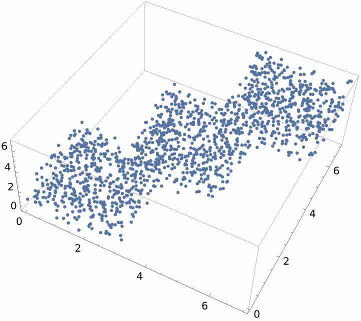 |
Visualize this dataset reduced to two dimensions:
| In[4]:= |
| Out[4]= |  |
MultidimensionalScaling will reduce to any dimension that is no larger than the input dimension. Here data is created in 10-dimensional space and visualized in three dimensions:
| In[5]:= | ![dim = 10;
num = 500;
vectors = Join[RandomReal[{0, 3}, {num, dim}], RandomReal[{2, 5}, {num, dim}],
RandomReal[{4, 7}, {num, dim}]];](https://www.wolframcloud.com/obj/resourcesystem/images/6a4/6a4a06f4-b0fe-4509-8484-35ec1440fffe/394139c61dfe5ea8.png) |
| In[6]:= |
| Out[6]= | 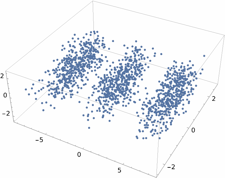 |
As is done in the reference page for DimensionReduce, load the Fisher Iris dataset from ExampleData:
| In[7]:= |
Reduce the dimension of the features:
| In[8]:= |
Group the examples by their species:
| In[9]:= |
Visualize the reduced dataset:
| In[10]:= |
| Out[10]= | 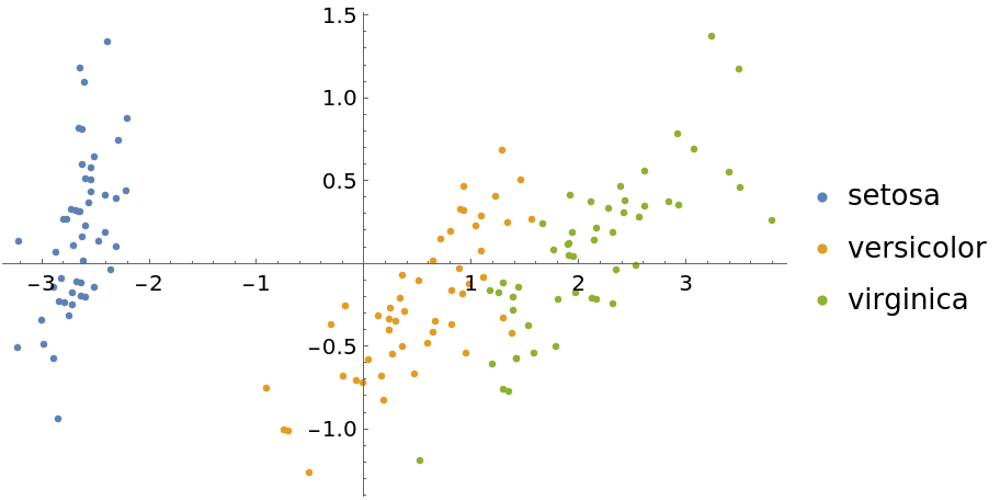 |
Now show some DimensionReduce methods for this same dataset. First, use the "PrincipalComponentsAnalysis" method:
| In[11]:= | ![featuresPCA = DimensionReduce[iris[[All, 1]], 2, Method -> "PrincipalComponentsAnalysis"];
byspeciesPCA = GroupBy[Thread[featuresPCA -> iris[[All, 2]]], Last -> First];
ListPlot[Values[byspeciesPCA], PlotLegends -> Keys[byspeciesPCA]]](https://www.wolframcloud.com/obj/resourcesystem/images/6a4/6a4a06f4-b0fe-4509-8484-35ec1440fffe/5422e580c2483c8c.png) |
| Out[12]= | 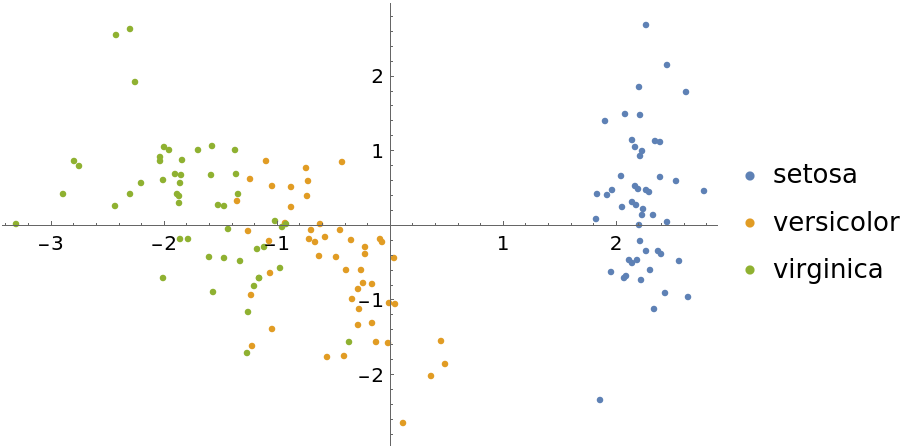 |
Use the "TSNE" method:
| In[13]:= | ![featuresTSNE = DimensionReduce[iris[[All, 1]], 2, Method -> "TSNE"];
byspeciesTSNE = GroupBy[Thread[featuresTSNE -> iris[[All, 2]]], Last -> First];
ListPlot[Values[byspeciesTSNE], PlotLegends -> Keys[byspeciesTSNE]]](https://www.wolframcloud.com/obj/resourcesystem/images/6a4/6a4a06f4-b0fe-4509-8484-35ec1440fffe/3413ffcab6643f9e.png) |
| Out[14]= | 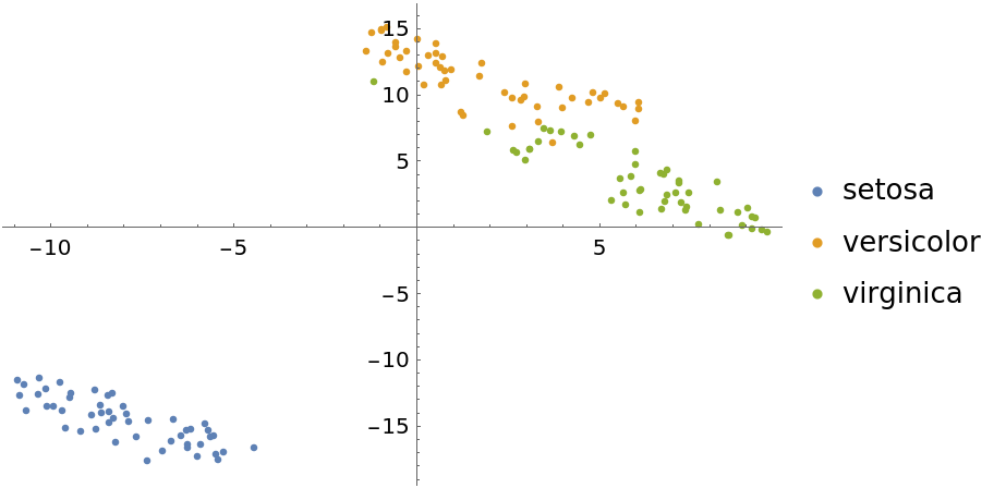 |
Visualize with the "LatentSemanticAnalysis" method:
| In[15]:= | ![featuresLSA = DimensionReduce[iris[[All, 1]], 2, Method -> "LatentSemanticAnalysis"];
byspeciesLSA = GroupBy[Thread[featuresLSA -> iris[[All, 2]]], Last -> First];
ListPlot[Values[byspeciesLSA], PlotLegends -> Keys[byspeciesLSA]]](https://www.wolframcloud.com/obj/resourcesystem/images/6a4/6a4a06f4-b0fe-4509-8484-35ec1440fffe/01069848f6a2fc74.png) |
| Out[16]= | 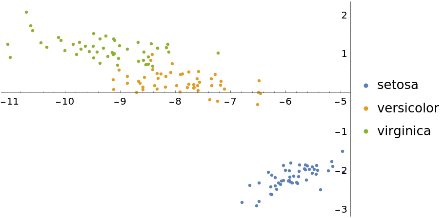 |
The "LatentSemanticAnalysis" method can be attained directly using SingularValueDecomposition:
| In[17]:= |
| In[18]:= | ![featuresLSA2 = LSA[iris[[All, 1]], 2];
byspeciesLSA2 = GroupBy[Thread[featuresLSA2 -> iris[[All, 2]]], Last -> First];
ListPlot[Values[byspeciesLSA2], PlotLegends -> Keys[byspeciesLSA2]]](https://www.wolframcloud.com/obj/resourcesystem/images/6a4/6a4a06f4-b0fe-4509-8484-35ec1440fffe/0653c9428b2d7966.png) |
| Out[19]= | 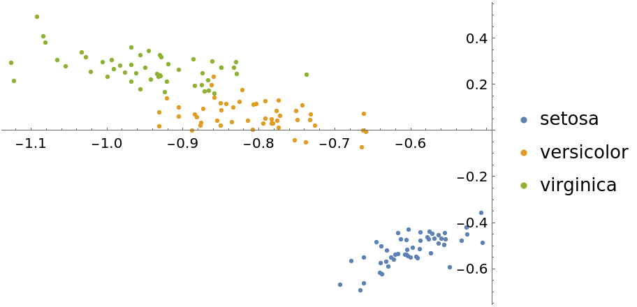 |
Illustrate multidimensional scaling on textual data using several popular literature texts from ExampleData:

Break each text into chunks of equal string length:

Find the most common words across all texts:

Create common word frequency vectors for each chunk:

Weight the frequency vectors using the log-entropy method:

Show the result of multidimensional scaling in two dimensions, grouping text chunks by position of the title in the list of text names:
| In[20]:= | ![wdim2 = ResourceFunction[
"MultidimensionalScaling", ResourceSystemBase -> "https://www.wolframcloud.com/obj/resourcesystem/api/1.0"][weightedWordsByChunkMatrix, 2];
byAuthorW = GatherBy[Thread[labels -> wdim2], First];
ListPlot[Values[byAuthorW], PlotLegends -> Apply[Union, Keys[byAuthorW]]]](https://www.wolframcloud.com/obj/resourcesystem/images/6a4/6a4a06f4-b0fe-4509-8484-35ec1440fffe/0d17f6470431a29f.png) |
| Out[22]= | 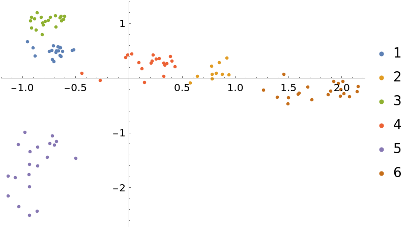 |
This work is licensed under a Creative Commons Attribution 4.0 International License