Wolfram Function Repository
Instant-use add-on functions for the Wolfram Language
Function Repository Resource:
Reduce a matrix of real values to low dimension using the principal coordinates analysis method
|
ResourceFunction["MultidimensionalScaling"][vecs,dim] uses principal coordinates analysis to find a "best projection" of vecs to dimension dim. |
|
|
ResourceFunction["MultidimensionalScaling"][vecs] projects vecs to two dimensions. |
Reduce the dimension of some vectors:
| In[1]:= |
|
| Out[1]= |
|
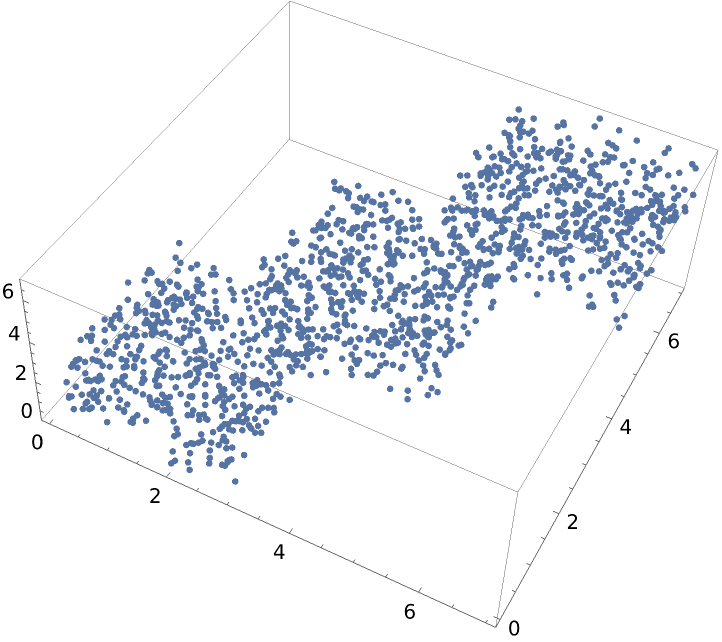
Create and visualize random 3D vectors:
| In[2]:= |
![vectors = Join[RandomReal[{0, 3}, {500, 3}], RandomReal[{2, 5}, {500, 3}], RandomReal[{4, 7}, {500, 3}]];
ListPointPlot3D[vectors]](https://www.wolframcloud.com/obj/resourcesystem/images/6a4/6a4a06f4-b0fe-4509-8484-35ec1440fffe/1-0-2/677efc7e8ab54777.png)
|
| Out[3]= |
|
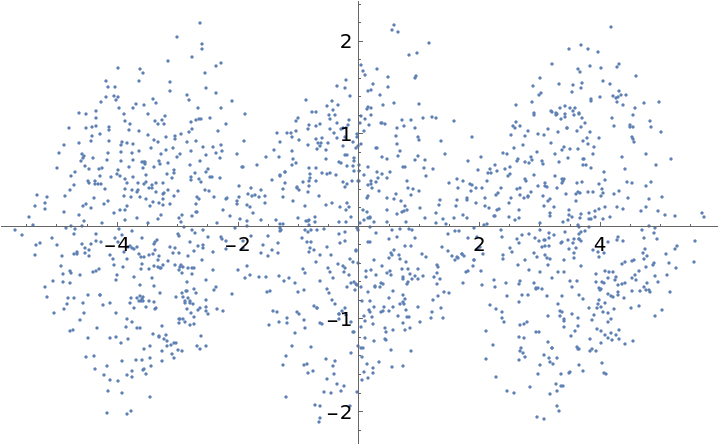
Visualize this dataset reduced to two dimensions:
| In[4]:= |
|
| Out[4]= |
|
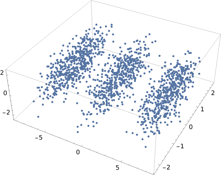
MultidimensionalScaling will reduce to any dimension that is no larger than the input dimension. Here we create data in ten dimensional space, and visualize in three dimensions:
| In[5]:= |
![dim = 10;
num = 500;
vectors = Join[RandomReal[{0, 3}, {num, dim}], RandomReal[{2, 5}, {num, dim}],
RandomReal[{4, 7}, {num, dim}]];](https://www.wolframcloud.com/obj/resourcesystem/images/6a4/6a4a06f4-b0fe-4509-8484-35ec1440fffe/1-0-2/69e9b5d8ca22470b.png)
|
| In[6]:= |
|
| Out[6]= |
|
As is done in the reference page for DimensionReduce, load the Fisher iris dataset from ExampleData:
| In[7]:= |
|
Reduce the dimension of the features:
| In[8]:= |
|
Group the examples by their species:
| In[9]:= |
|
Visualize the reduced dataset:
| In[10]:= |
|
| Out[10]= |
|
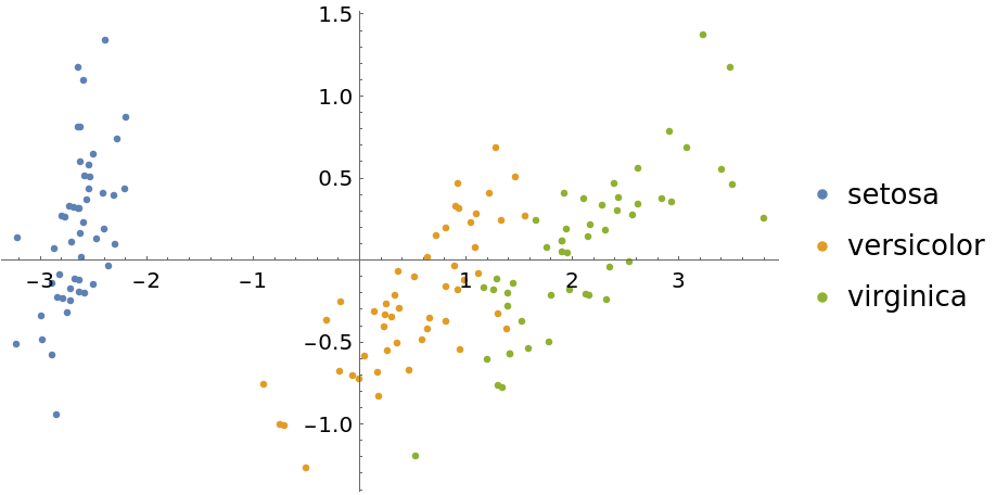
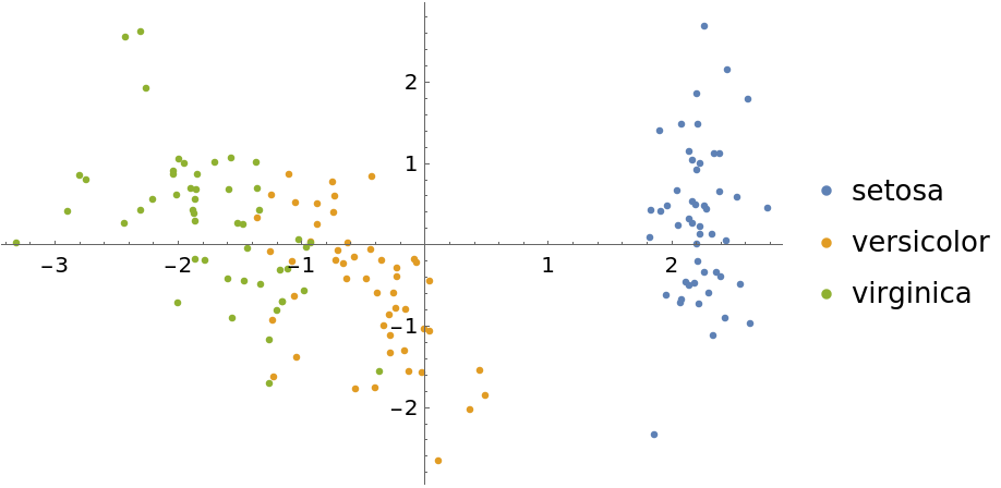
Now show some DimensionReduce methods for this same dataset. First we use the "PrincipalComponentsAnalysis" method:
| In[11]:= |
![featuresPCA = DimensionReduce[iris[[All, 1]], 2, Method -> "PrincipalComponentsAnalysis"];
byspeciesPCA = GroupBy[Thread[featuresPCA -> iris[[All, 2]]], Last -> First];
ListPlot[Values[byspeciesPCA], PlotLegends -> Keys[byspeciesPCA]]](https://www.wolframcloud.com/obj/resourcesystem/images/6a4/6a4a06f4-b0fe-4509-8484-35ec1440fffe/1-0-2/608a95d00fead564.png)
|
| Out[12]= |
|
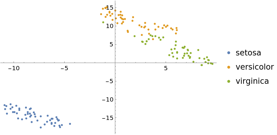
Use the "TSNE" method:
| In[13]:= |
![featuresTSNE = DimensionReduce[iris[[All, 1]], 2, Method -> "TSNE"];
byspeciesTSNE = GroupBy[Thread[featuresTSNE -> iris[[All, 2]]], Last -> First];
ListPlot[Values[byspeciesTSNE], PlotLegends -> Keys[byspeciesTSNE]]](https://www.wolframcloud.com/obj/resourcesystem/images/6a4/6a4a06f4-b0fe-4509-8484-35ec1440fffe/1-0-2/5a1af860fe7b67a1.png)
|
| Out[14]= |
|
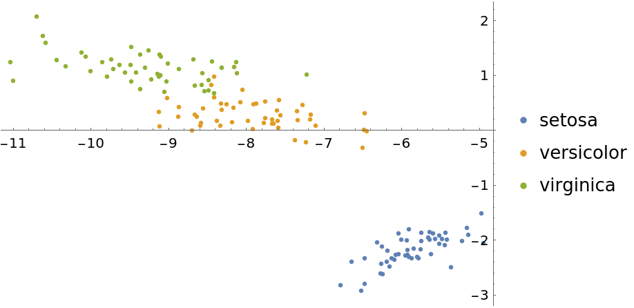
Visualize with the "LatentSemanticAnalysis" method:
| In[15]:= |
![featuresLSA = DimensionReduce[iris[[All, 1]], 2, Method -> "LatentSemanticAnalysis"];
byspeciesLSA = GroupBy[Thread[featuresLSA -> iris[[All, 2]]], Last -> First];
ListPlot[Values[byspeciesLSA], PlotLegends -> Keys[byspeciesLSA]]](https://www.wolframcloud.com/obj/resourcesystem/images/6a4/6a4a06f4-b0fe-4509-8484-35ec1440fffe/1-0-2/5f63cfa4c9d5b84a.png)
|
| Out[16]= |
|
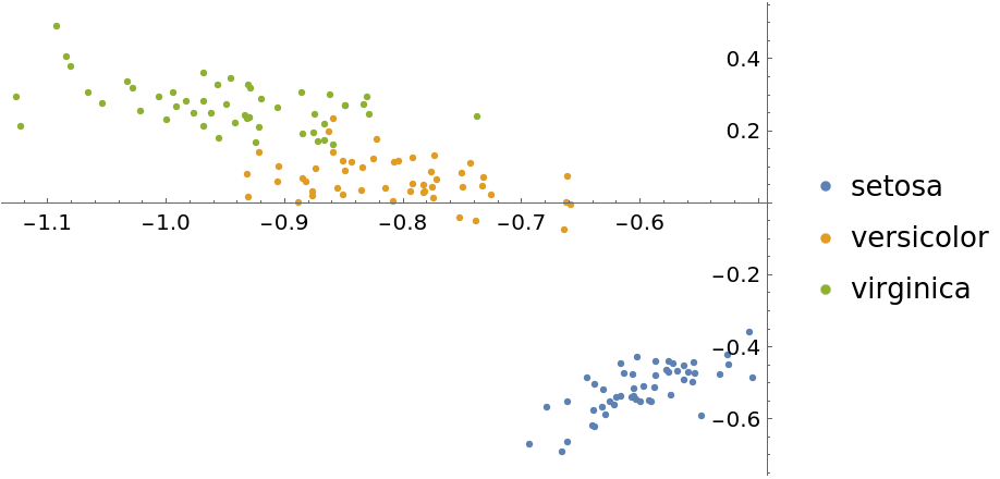
The "LatentSemanticAnalysis" method can be attained directly using SingularValueDecomposition:
| In[17]:= |
|
| In[18]:= |
![featuresLSA2 = LSA[iris[[All, 1]], 2];
byspeciesLSA2 = GroupBy[Thread[featuresLSA2 -> iris[[All, 2]]], Last -> First];
ListPlot[Values[byspeciesLSA2], PlotLegends -> Keys[byspeciesLSA2]]](https://www.wolframcloud.com/obj/resourcesystem/images/6a4/6a4a06f4-b0fe-4509-8484-35ec1440fffe/1-0-2/16aa96326f51747a.png)
|
| Out[19]= |
|
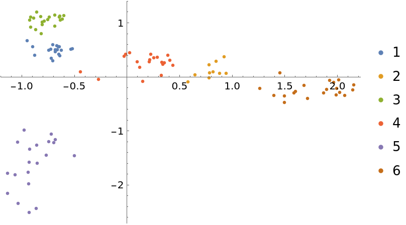
Illustrate multidimensional scaling on textual data using several popular literature texts from ExampleData:

Break each text into chunks of equal string length:

Find the most common words across all texts:

Create common word frequency vectors for each chunk:

Weight the frequency vectors using the log-entropy method:

Show the result of multidimensional scaling in two dimensions, grouping text chunks by position of title in the list of text names:
| In[20]:= |
![wdim2 = ResourceFunction["MultidimensionalScaling"][
weightedWordsByChunkMatrix, 2];
byAuthorW = GatherBy[Thread[labels -> wdim2], First];
ListPlot[Values[byAuthorW], PlotLegends -> Apply[Union, Keys[byAuthorW]]]](https://www.wolframcloud.com/obj/resourcesystem/images/6a4/6a4a06f4-b0fe-4509-8484-35ec1440fffe/1-0-2/2d5bb439b2e44880.png)
|
| Out[22]= |
|
This work is licensed under a Creative Commons Attribution 4.0 International License