Details and Options
ResourceFunction["PhylogeneticTreePlot"] uses an alignment-free method to compare pairs of sequences.
Input sequences should be strings comprised of the standard nucleotide letters {A,C,G,T}. Lowercase letters are also allowed. The character U is allowed and is replaced by T. All other characters, such as N, are removed.
ResourceFunction["PhylogeneticTreePlot"] uses
Dendrogram and accepts all options for that function.
Most default option settings agree with those of
Dendrogram.
ResourceFunction["PhylogeneticTreePlot"] creates the dendrogram from vectors that are derived via dimensional reductions of the input genetic sequences.
By default, each sequence is first converted to an image using the Frequency Chaos Game Representation (FCGR).
FCGR images are reduced in dimension using a Fourier Cosine Transform (FCT). A further dimensional reduction is done using the Singular Value Decomposition (SVD) on vectors comprised of the flattened FCT matrices.
An explanation may be found in the articles noted in the Related Links and Source Metadata sections.
The dimensional reduction described above has certain parameters that in principle might be changed. ResourceFunction["PhylogeneticTreePlot"] uses a fixed set of values for these that has been seen to perform fairly well in practice.
In order to produce a reasonable grouping, ResourceFunction["PhylogeneticTreePlot"] requires moderately long genetic sequences containing at least a few thousand nucleotides.
The SVD step of the dimension reduction, when applied to vectors that came from a set of very similar genome sequences, will tend to give a result where the reduced vectors are dominated by a large first value that is approximately equal across the set. This tends to distort the distances between genomes. The option
"IgnoreOutlier" (default:
Automatic) is provided to address this. The automatic behavior is to remove the first components whenever the largest singular value is at least ten times the size of the next largest.
ResourceFunction["PhylogeneticTreePlot"] takes an option
"VectorMethod". The
Automatic default converts sequences to vectors using the methodology described above. A user-defined method can be specified with this option. One possibility is to use the resource function
StringsToVectors.

![genomesMammal = {"V00662", "D38116", "D38113", "D38114", "X99256", "Y18001", "AY863426", "D38115", "NC_002083", "U20753", "U96639", "AJ002189", "AF010406", "AF533441", "V00654", "AY488491", "EU442884", "EF551003", "EF551002", "X97336", "Y07726", "DQ402478",
"AF303110", "AF303111", "EF212882", "AJ001588", "X88898", "NC_002764", "AJ238588", "AJ001562", "X72204", "NC_005268", "NC_007441", "NC_008830", "NC_001788", "NC_001321", "NC_005270", "NC_001640", "NC_005275", "NC_006931", "NC_010640"};
speciesMammal = {"Human", "Pygmy chimpanzee", "Common chimpanzee", "Gorilla", "Gibbon", "Baboon", "Vervet monkey", "Bornean orangutan", "Sumatran orangutan", "Cat", "Dog", "Pig", "Sheep", "Goat", "Cow", "Buffalo", "Wolf", "Tiger", "Leopard", "Indian rhinoceros", "White rhinoceros", "Black bear", "Brown bear", "Polar bear", "Giant panda", "Rabbit", "Hedgehog", "Macaca thibet", "Squirrel", "Dormouse", "Blue whale", "Bowhead whale", "Chiru", "Common warthog", "Donkey", "Fin whale", "Gray whale", "Horse", "Indus river dolphin", "North pacific right whale", "Taiwan serow"};
stringColor[str_String] := Which[
StringContainsQ[str, {"Human", "chimpanzee", "Gorilla", "orangutan"}],
Red,
StringContainsQ[str, {"Gibbon", "Baboon", "monkey", "thibet"}], Orange,
StringContainsQ[str, {"Tiger", "Leopard", "Cat"}],
Darker[Green],
StringContainsQ[str, {"Dog", "Wolf"}],
Lighter[Green],
StringContainsQ[
str, {"Cow", "Buffalo", "Goat", "Sheep", "Chiru", "serow"}],
Darker[Brown],
StringContainsQ[str, "rhino"],
Lighter[Brown],
StringContainsQ[str, {"bear", "panda"}], Black,
StringContainsQ[str, {"mouse", "Squirrel", "Rabbit"}], Gray,
StringContainsQ[str, {"Pig", "warthog"}],
Darker[Blue],
StringContainsQ[str, {"Donkey", "Horse"}], Blue,
StringContainsQ[str, {"whale", "dolphin"}], Purple,
StringContainsQ[str, "Hedgehog"],
Darker[Gray]]
speciesMammalColored = Map[Style[#, stringColor[#]] &, speciesMammal]](https://www.wolframcloud.com/obj/resourcesystem/images/562/562d05d8-fc55-4fe9-beb8-4e6746b1f1da/6212a2167e78ab52.png)
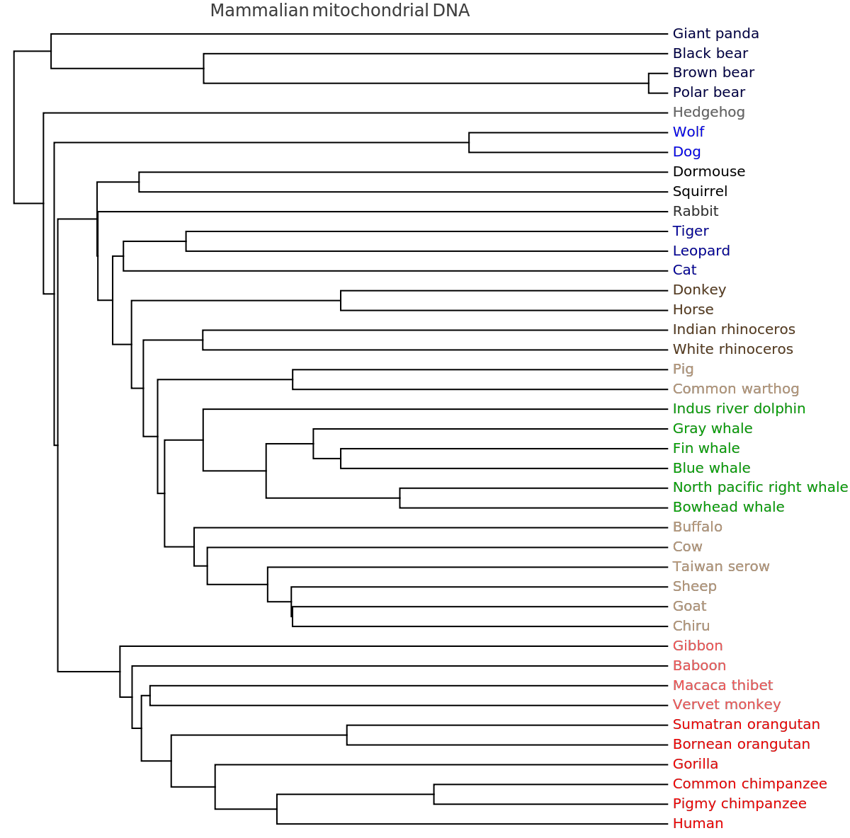
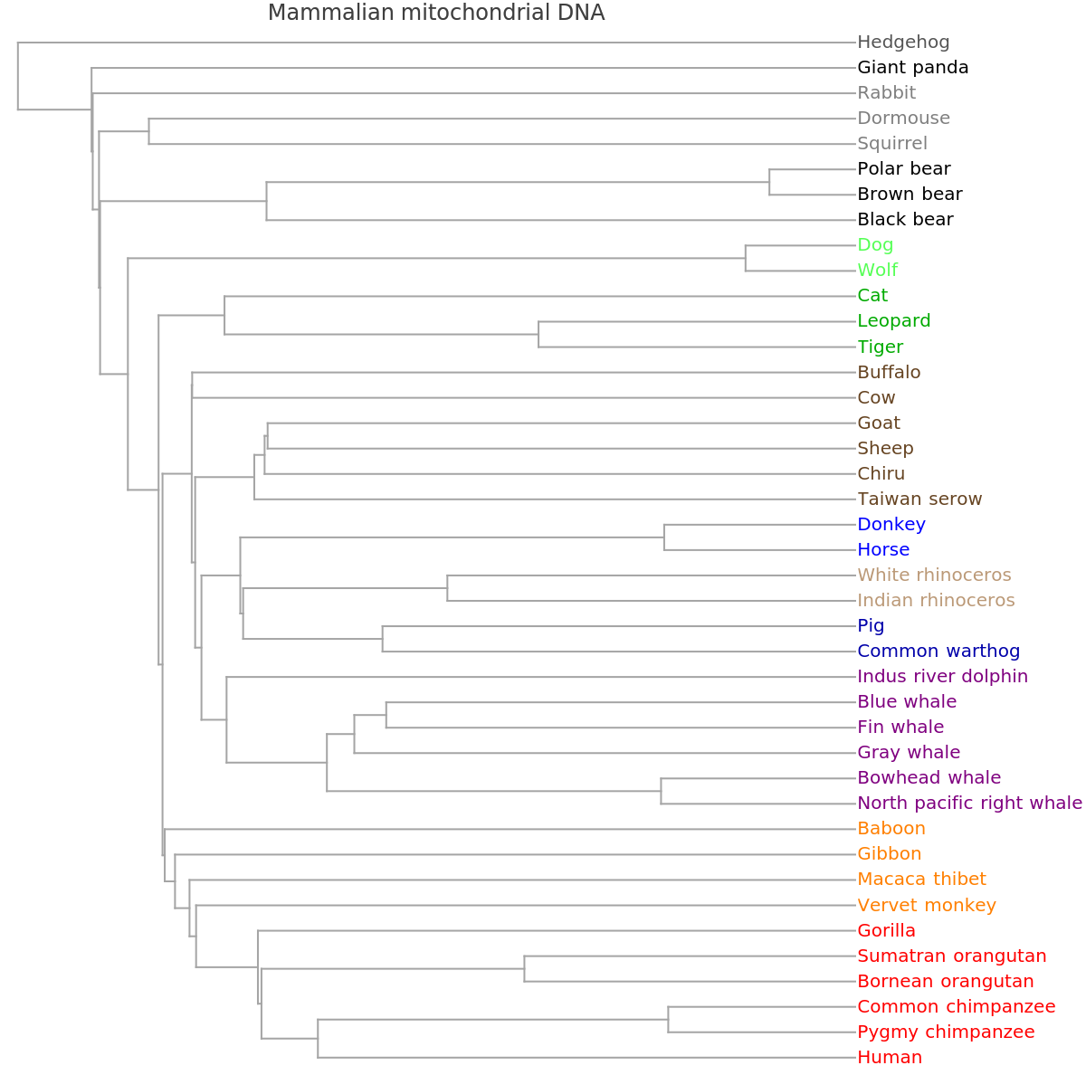
![ResourceFunction[
"PhylogeneticTreePlot", ResourceSystemBase -> "https://www.wolframcloud.com/obj/resourcesystem/api/1.0"][sequencesMammal, speciesMammalColored, PlotLabel -> "Mammalian mitochondrial DNA"]](https://www.wolframcloud.com/obj/resourcesystem/images/562/562d05d8-fc55-4fe9-beb8-4e6746b1f1da/603b368a2b777385.png)
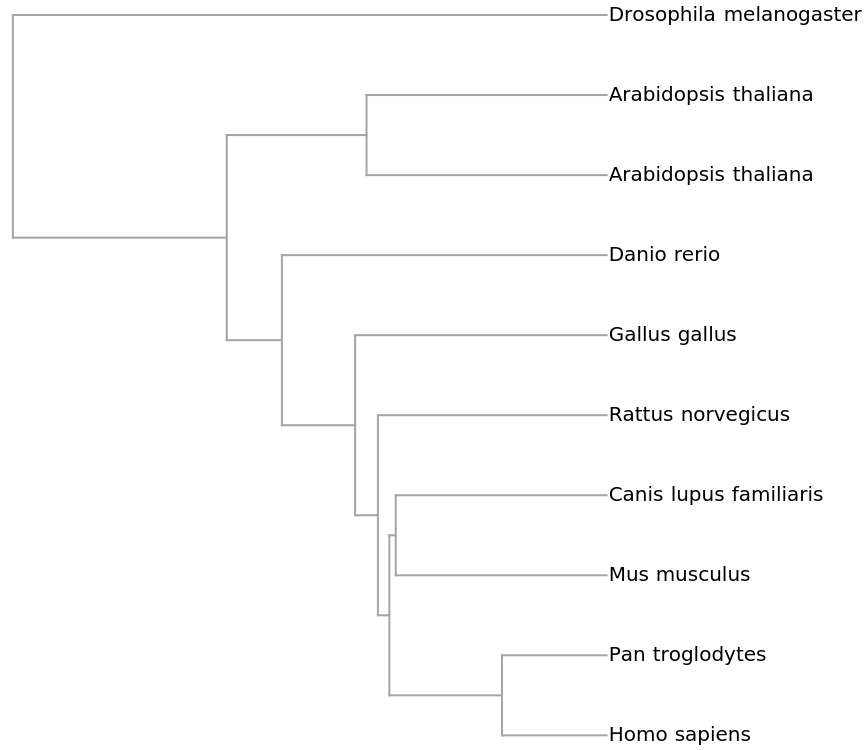
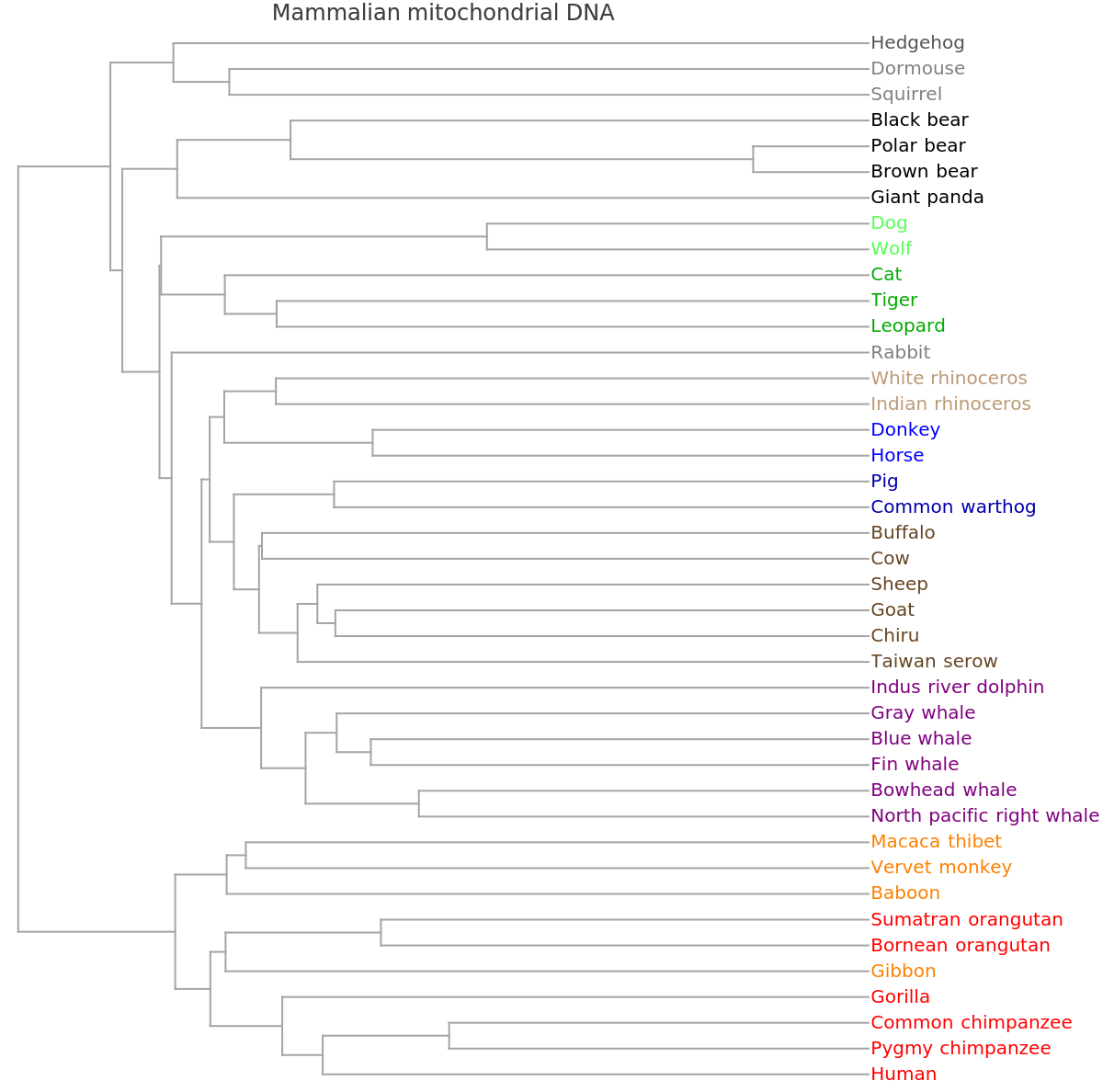
![ResourceFunction[
"PhylogeneticTreePlot", ResourceSystemBase -> "https://www.wolframcloud.com/obj/resourcesystem/api/1.0"][sequencesMammal, speciesMammalColored, PlotLabel -> "Mammalian mitochondrial DNA", ClusterDissimilarityFunction -> "Average"]](https://www.wolframcloud.com/obj/resourcesystem/images/562/562d05d8-fc55-4fe9-beb8-4e6746b1f1da/12c7f5f1971a91bc.png)
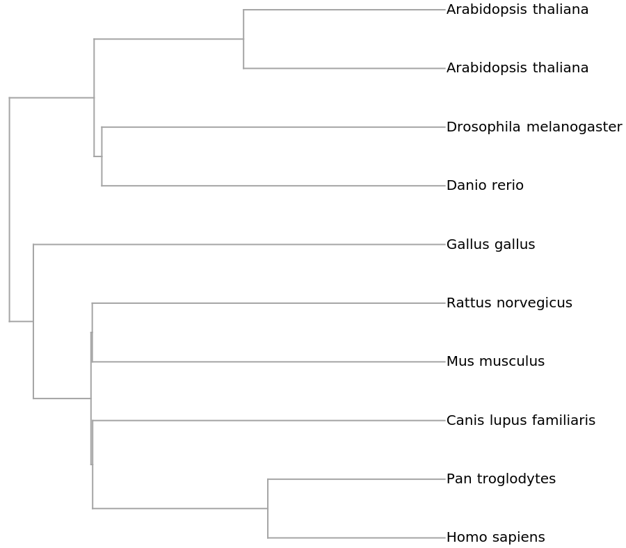
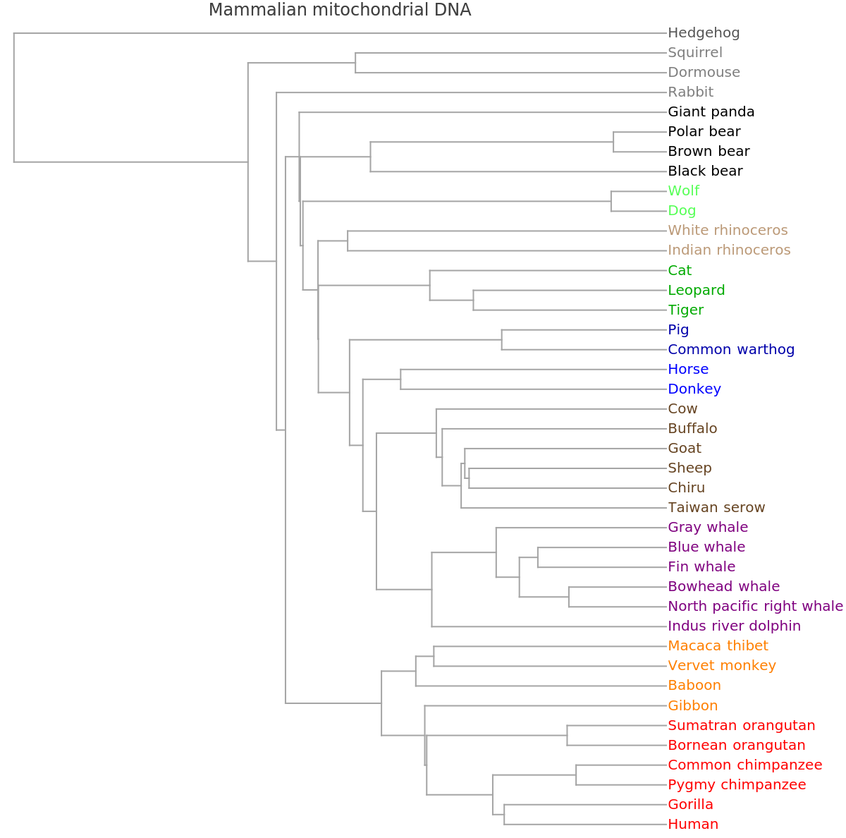
![ResourceFunction[
"PhylogeneticTreePlot", ResourceSystemBase -> "https://www.wolframcloud.com/obj/resourcesystem/api/1.0"][sequencesMammal, speciesMammalColored, "VectorMethod" -> ResourceFunction["StringsToVectors"], PlotLabel -> "Mammalian mitochondrial DNA"]](https://www.wolframcloud.com/obj/resourcesystem/images/562/562d05d8-fc55-4fe9-beb8-4e6746b1f1da/1ef3fe8c48240b0a.png)
![fullGenes = ResourceData["Genetic Sequences for the SARS-CoV-2 Coronavirus"][
Select[StringContainsQ[#GenBankTitle, "complete genome"] && FreeQ[#CollectionDate, Missing] && Head[#CollectionDate] === DateObject && FreeQ[#GeographicLocation, Missing] &], {"Sequence", "GeographicLocation", "CollectionDate", "Accession", "GenBankTitle"}];
geneLists = Normal[fullGenes];
geneLists // Length](https://www.wolframcloud.com/obj/resourcesystem/images/562/562d05d8-fc55-4fe9-beb8-4e6746b1f1da/27b317c3e0e93fc5.png)
![dropTrailingA[seq_] := StringReplace[seq, StartOfString ~~ Shortest[a__] ~~ ("A" ..) ~~ EndOfString :> a];
normalGL = Map[Values, geneListsAbbrev];
midsize = Select[normalGL, 29825 <= StringLength[dropTrailingA[#[[1]]]] <= 29885 &];
{fullseqs0, places, dates} = Transpose[midsize[[All, 1 ;; 3]]];
fullseqs = Map[dropTrailingA, fullseqs0];
fullseqs // Length](https://www.wolframcloud.com/obj/resourcesystem/images/562/562d05d8-fc55-4fe9-beb8-4e6746b1f1da/2f3841701a7f56e0.png)
![dates1 = Map[First, dates];
ndates1 = Map[(#[[1]] - 2019)*365 + #[[2]]*30.4 + If[Length[#] == 3, #[[3]], 15] &, dates1];
ndates = Rescale[ndates1];
colorDateLabels = Thread[Style[dates1, Map[Darker[Hue[#]] &, ndates + .05]]];
placeNames = Map[If[Head[#] === Entity, #[[2]], Head[#]] &, places];
placeSet = Union[placeNames];
nplaces = Length[placeSet];
crange = Range[nplaces]/(nplaces + 1);
biggest = Ordering[
Map[Length, Map[ColorData[#, "ColorList"] &, ColorData["Indexed"]]], -1];
placeColors = Take[Cases[
ColorData[ColorData["Indexed"][[biggest[[1]]]], "ColorList"], _RGBColor], UpTo[nplaces]];
colorPlaceRule = Thread[placeSet -> placeColors];
colorPlaceLabels = Thread[Style[placeNames, placeNames /. colorPlaceRule]];
colorPlaceDateLabels = Thread[{colorPlaceLabels, colorDateLabels}];](https://www.wolframcloud.com/obj/resourcesystem/images/562/562d05d8-fc55-4fe9-beb8-4e6746b1f1da/43eadd37afdbca2d.png)
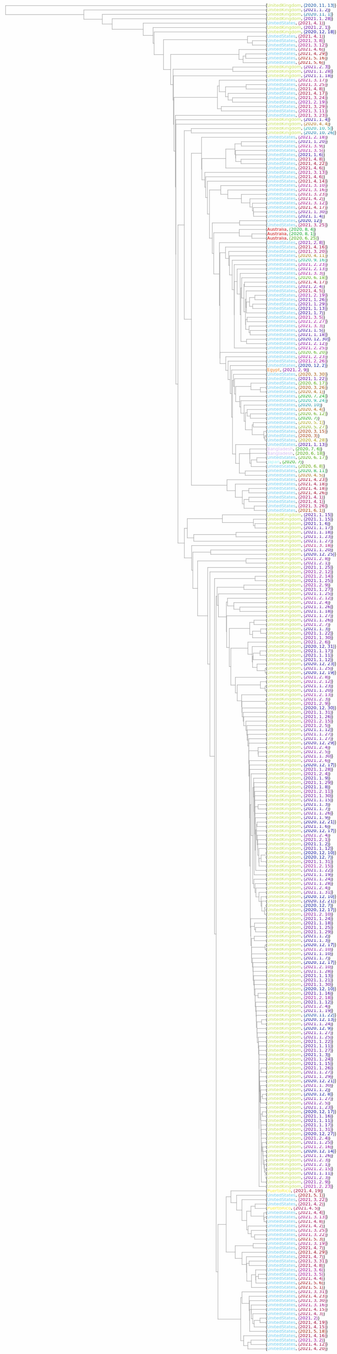
![Options[OldPhylogeneticTreePlot] = Join[Options[
HierarchicalClustering`DendrogramPlot], {AspectRatio -> 1.2, ImageSize -> 600, "IgnoreOutlier" -> Automatic}] /. (HierarchicalClustering`Orientation -> aa_) :> (HierarchicalClustering`Orientation -> Left);
OldPhylogeneticTreePlot[geneseqs_, labels_, opts : OptionsPattern[]] :=
OldPhylogeneticTreePlot[geneseqs, labels, "", opts]
OldPhylogeneticTreePlot[geneseqs_, labels_, plabel_, opts : OptionsPattern[]] := With[{freq = 30, keep = 40, dim = 7},
Module[
{ftts, vecs, ratio, size, io, optsd},
{ratio, size, io} = ({AspectRatio, ImageSize, "IgnoreOutlier"} /. {opts}) /. Thread[{AspectRatio, ImageSize, "IgnoreOutlier"} -> {OptionValue[AspectRatio], OptionValue[ImageSize], OptionValue["IgnoreOutlier"]}];
Block[{$ContextPath}, Needs["HierarchicalClustering`"]];
optsd = FilterRules[{opts}, Options[HierarchicalClustering`DendrogramPlot]];
ftts = Map[Developer`ToPackedArray[
processNucleotideString[#, dim, freq]] &, geneseqs];
vecs = FTTsToVectors[ftts, keep, io];
HierarchicalClustering`DendrogramPlot[vecs, HierarchicalClustering`LeafLabels -> labels, PlotLabel -> plabel, AspectRatio -> ratio, ImageSize -> size, Apply[Sequence, optsd], Apply[Sequence, Options[
ResourceFunction[
"PhylogeneticTreePlot", ResourceSystemBase -> "https://www.wolframcloud.com/obj/resourcesystem/api/1.0"]]]]
]]](https://www.wolframcloud.com/obj/resourcesystem/images/562/562d05d8-fc55-4fe9-beb8-4e6746b1f1da/0909fb9c8a9ae6b9.png)
![genomesMammal = {"V00662", "D38116", "D38113", "D38114", "X99256", "Y18001", "AY863426", "D38115", "NC_002083", "U20753", "U96639", "AJ002189", "AF010406", "AF533441", "V00654", "AY488491", "EU442884", "EF551003", "EF551002", "X97336", "Y07726", "DQ402478", "AF303110", "AF303111", "EF212882", "AJ001588", "X88898", "NC_002764", "AJ238588", "AJ001562", "X72204", "NC_005268", "NC_007441", "NC_008830", "NC_001788", "NC_001321", "NC_005270", "NC_001640", "NC_005275", "NC_006931", "NC_010640"};
speciesMammalColored = {\!\(\*
StyleBox["\"\<Human\>\"",
StripOnInput->False,
FontColor->RGBColor[1, 0, 0],
"NodeID" -> 114]\), \!\(\*
StyleBox["\"\<Pigmy chimpanzee\>\"",
StripOnInput->False,
FontColor->RGBColor[1, 0, 0],
"NodeID" -> 115]\), \!\(\*
StyleBox["\"\<Common chimpanzee\>\"",
StripOnInput->False,
FontColor->RGBColor[1, 0, 0],
"NodeID" -> 116]\), \!\(\*
StyleBox["\"\<Gorilla\>\"",
StripOnInput->False,
FontColor->RGBColor[1, 0, 0],
"NodeID" -> 117]\), \!\(\*
StyleBox["\"\<Gibbon\>\"",
StripOnInput->False,
FontColor->RGBColor[1,
Rational[1, 3],
Rational[1, 3]],
"NodeID" -> 118]\), \!\(\*
StyleBox["\"\<Baboon\>\"",
StripOnInput->False,
FontColor->RGBColor[1,
Rational[1, 3],
Rational[1, 3]],
"NodeID" -> 119]\), \!\(\*
StyleBox["\"\<Vervet monkey\>\"",
StripOnInput->False,
FontColor->RGBColor[1,
Rational[1, 3],
Rational[1, 3]],
"NodeID" -> 120]\), \!\(\*
StyleBox["\"\<Bornean orangutan\>\"",
StripOnInput->False,
FontColor->RGBColor[1, 0, 0],
"NodeID" -> 121]\), \!\(\*
StyleBox["\"\<Sumatran orangutan\>\"",
StripOnInput->False,
FontColor->RGBColor[1, 0, 0],
"NodeID" -> 122]\), \!\(\*
StyleBox["\"\<Cat\>\"",
StripOnInput->False,
FontColor->RGBColor[0., 0., 0.65],
"NodeID" -> 123]\), \!\(\*
StyleBox["\"\<Dog\>\"",
StripOnInput->False,
FontColor->RGBColor[0, 0, 1],
"NodeID" -> 124]\), \!\(\*
StyleBox["\"\<Pig\>\"",
StripOnInput->False,
FontColor->RGBColor[0.7333333333333333, 0.6, 0.4666666666666667],
"NodeID" -> 125]\), \!\(\*
StyleBox["\"\<Sheep\>\"",
StripOnInput->False,
FontColor->RGBColor[0.7333333333333333, 0.6, 0.4666666666666667],
"NodeID" -> 126]\), \!\(\*
StyleBox["\"\<Goat\>\"",
StripOnInput->False,
FontColor->RGBColor[0.7333333333333333, 0.6, 0.4666666666666667],
"NodeID" -> 127]\), \!\(\*
StyleBox["\"\<Cow\>\"",
StripOnInput->False,
FontColor->RGBColor[0.7333333333333333, 0.6, 0.4666666666666667],
"NodeID" -> 128]\), \!\(\*
StyleBox["\"\<Buffalo\>\"",
StripOnInput->False,
FontColor->RGBColor[0.7333333333333333, 0.6, 0.4666666666666667],
"NodeID" -> 129]\), \!\(\*
StyleBox["\"\<Wolf\>\"",
StripOnInput->False,
FontColor->RGBColor[0, 0, 1],
"NodeID" -> 130]\), \!\(\*
StyleBox["\"\<Tiger\>\"",
StripOnInput->False,
FontColor->RGBColor[0., 0., 0.65],
"NodeID" -> 131]\), \!\(\*
StyleBox["\"\<Leopard\>\"",
StripOnInput->False,
FontColor->RGBColor[0., 0., 0.65],
"NodeID" -> 132]\), \!\(\*
StyleBox["\"\<Indian rhinoceros\>\"",
StripOnInput->False,
FontColor->RGBColor[0.36, 0.24, 0.12],
"NodeID" -> 133]\), \!\(\*
StyleBox["\"\<White rhinoceros\>\"",
StripOnInput->False,
FontColor->RGBColor[0.36, 0.24, 0.12],
"NodeID" -> 134]\), \!\(\*
StyleBox["\"\<Black bear\>\"",
StripOnInput->False,
FontColor->RGBColor[0., 0., 0.30000000000000004`],
"NodeID" -> 135]\), \!\(\*
StyleBox["\"\<Brown bear\>\"",
StripOnInput->False,
FontColor->RGBColor[0., 0., 0.30000000000000004`],
"NodeID" -> 136]\), \!\(\*
StyleBox["\"\<Polar bear\>\"",
StripOnInput->False,
FontColor->RGBColor[0., 0., 0.30000000000000004`],
"NodeID" -> 137]\), \!\(\*
StyleBox["\"\<Giant panda\>\"",
StripOnInput->False,
FontColor->RGBColor[0., 0., 0.30000000000000004`],
"NodeID" -> 138]\), \!\(\*
StyleBox["\"\<Rabbit\>\"",
StripOnInput->False,
FontColor->RGBColor[0.2, 0.2, 0.2],
"NodeID" -> 139]\), \!\(\*
StyleBox["\"\<Hedgehog\>\"",
StripOnInput->False,
FontColor->RGBColor[0.4, 0.4, 0.4],
"NodeID" -> 140]\), \!\(\*
StyleBox["\"\<Macaca thibet\>\"",
StripOnInput->False,
FontColor->RGBColor[1,
Rational[1, 3],
Rational[1, 3]],
"NodeID" -> 141]\), \!\(\*
StyleBox["\"\<Squirrel\>\"",
StripOnInput->False,
FontColor->GrayLevel[0],
"NodeID" -> 142]\), \!\(\*
StyleBox["\"\<Dormouse\>\"",
StripOnInput->False,
FontColor->GrayLevel[0],
"NodeID" -> 143]\), \!\(\*
StyleBox["\"\<Blue whale\>\"",
StripOnInput->False,
FontColor->RGBColor[0,
Rational[2, 3], 0],
"NodeID" -> 144]\), \!\(\*
StyleBox["\"\<Bowhead whale\>\"",
StripOnInput->False,
FontColor->RGBColor[0,
Rational[2, 3], 0],
"NodeID" -> 145]\), \!\(\*
StyleBox["\"\<Chiru\>\"",
StripOnInput->False,
FontColor->RGBColor[0.7333333333333333, 0.6, 0.4666666666666667],
"NodeID" -> 146]\), \!\(\*
StyleBox["\"\<Common warthog\>\"",
StripOnInput->False,
FontColor->RGBColor[0.7333333333333333, 0.6, 0.4666666666666667],
"NodeID" -> 147]\), \!\(\*
StyleBox["\"\<Donkey\>\"",
StripOnInput->False,
FontColor->RGBColor[0.36, 0.24, 0.12],
"NodeID" -> 148]\), \!\(\*
StyleBox["\"\<Fin whale\>\"",
StripOnInput->False,
FontColor->RGBColor[0,
Rational[2, 3], 0],
"NodeID" -> 149]\), \!\(\*
StyleBox["\"\<Gray whale\>\"",
StripOnInput->False,
FontColor->RGBColor[0,
Rational[2, 3], 0],
"NodeID" -> 150]\), \!\(\*
StyleBox["\"\<Horse\>\"",
StripOnInput->False,
FontColor->RGBColor[0.36, 0.24, 0.12],
"NodeID" -> 151]\), \!\(\*
StyleBox["\"\<Indus river dolphin\>\"",
StripOnInput->False,
FontColor->RGBColor[0,
Rational[2, 3], 0],
"NodeID" -> 152]\), \!\(\*
StyleBox["\"\<North pacific right whale\>\"",
StripOnInput->False,
FontColor->RGBColor[0,
Rational[2, 3], 0],
"NodeID" -> 153]\), \!\(\*
StyleBox["\"\<Taiwan serow\>\"",
StripOnInput->False,
FontColor->RGBColor[0.7333333333333333, 0.6, 0.4666666666666667],
"NodeID" -> 154]\)};
getFASTA = ResourceFunction["ImportFASTA"];
AbsoluteTiming[
sequencesMammal = Map[getFASTA, genomesMammal][[All, 2, 1]];]](https://www.wolframcloud.com/obj/resourcesystem/images/562/562d05d8-fc55-4fe9-beb8-4e6746b1f1da/56864a7fa32a7b6b.png)
![OldPhylogeneticTreePlot[sequencesMammal, speciesMammalColored, "Mammalian mitochondrial DNA", DistanceFunction -> CosineDistance]](https://www.wolframcloud.com/obj/resourcesystem/images/562/562d05d8-fc55-4fe9-beb8-4e6746b1f1da/008bebc0af60fecf.png)