Wolfram Function Repository
Instant-use add-on functions for the Wolfram Language
Function Repository Resource:
Generate the Steiner circumellipse of a 2D triangle
ResourceFunction["SteinerCircumellipse"][{p1,p2,p3}] returns an Ellipsoid representing the Steiner circumellipse of the triangle defined by vertices p1,p2 and p3. | |
ResourceFunction["SteinerCircumellipse"][{p1,p2,p3},property] gives the value of the specified property. |
| "Ellipsoid" | Ellipsoid representing the circumellipse |
| "Parametric" | parametric equation for the circumellipse as a pure function |
| "Implicit" | implicit Cartesian equation for the circumellipse as a pure function |
Show a triangle together with its Steiner circumellipse:
| In[1]:= | ![tri = {{0, 0}, {1.2, 4}, {5, 0}};
Graphics[{FaceForm[], {EdgeForm[Red], Triangle[tri]}, {EdgeForm[Blue],
ResourceFunction["SteinerCircumellipse"][tri]}}]](https://www.wolframcloud.com/obj/resourcesystem/images/cf0/cf01e293-cf19-4344-b7b1-bf0bb605974b/4724de42aba11c7a.png) |
| Out[1]= | 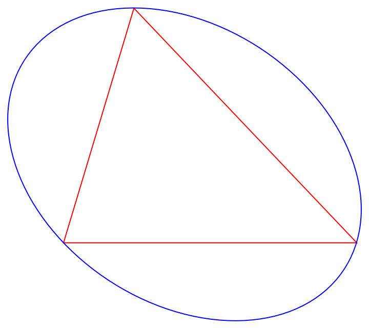 |
A triangle:
| In[2]:= |
| Out[2]= |  |
Generate the parametric equation of the triangle's Steiner circumellipse:
| In[3]:= |
| Out[3]= |
Plot the parametric equation along with the triangle:
| In[4]:= |
| Out[4]= | 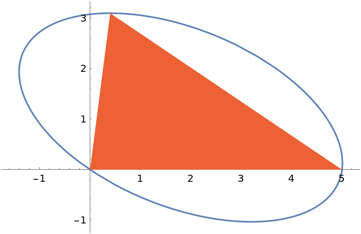 |
Generate the implicit equation of the triangle's Steiner circumellipse:
| In[5]:= |
| Out[5]= |
Plot the implicit equation along with the triangle:
| In[6]:= |
| Out[6]= | 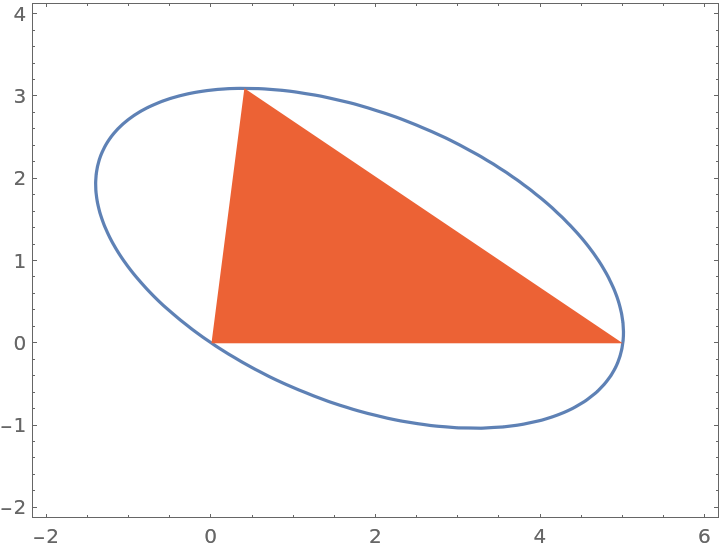 |
Use the resource function EllipseProperties to generate properties of the circumellipse:
| In[7]:= | ![ResourceFunction["EllipseProperties"][
ResourceFunction["SteinerCircumellipse"][{{0, 0}, {1.1, 4}, {5, 0}}, "Implicit"][x, y] == 0, {x, y}]](https://www.wolframcloud.com/obj/resourcesystem/images/cf0/cf01e293-cf19-4344-b7b1-bf0bb605974b/6df545f1f9870920.png) |
| Out[7]= |  |
The area of the Steiner circumellipse is a constant multiple of the area of the original triangle:
| In[8]:= | ![tri = Triangle[{{0, 0}, {1.5, 4}, {5, 0}}];
Area[ResourceFunction["SteinerCircumellipse"][tri]] - (4 \[Pi])/(
3 Sqrt[3]) Area[tri] // Chop](https://www.wolframcloud.com/obj/resourcesystem/images/cf0/cf01e293-cf19-4344-b7b1-bf0bb605974b/7c4eedf1c8900dd4.png) |
| Out[8]= |
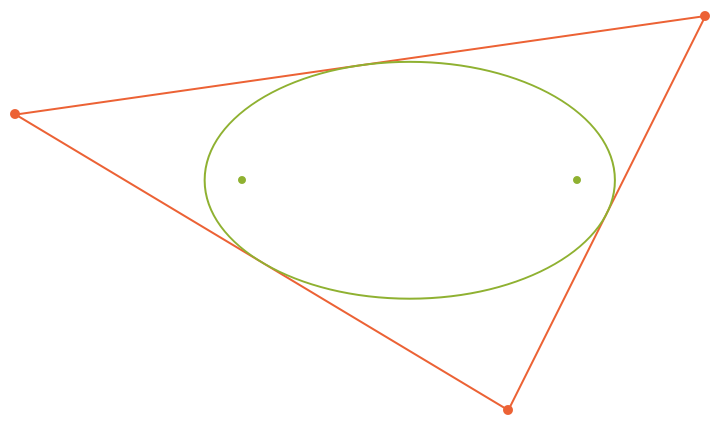
The Steiner inellipse is the Steiner circumellipse scaled by a factor of 1/2. It passes through the midpoints of the triangle's sides:
| In[9]:= | ![tri = Triangle[{{0, 0}, {1.5, 4}, {5, 0}}];
inell = TransformedRegion[
ResourceFunction["SteinerCircumellipse"][tri], ScalingTransform[{1/2, 1/2}, Mean @@ tri]];
Graphics[{FaceForm[], {EdgeForm[Blue], tri}, {EdgeForm[Red], inell}, {Brown, AbsolutePointSize[5], Point[Mean /@ Partition[First[tri], 2, 1, 1]]}}]](https://www.wolframcloud.com/obj/resourcesystem/images/cf0/cf01e293-cf19-4344-b7b1-bf0bb605974b/4215d8cede22c614.png) |
| Out[9]= | 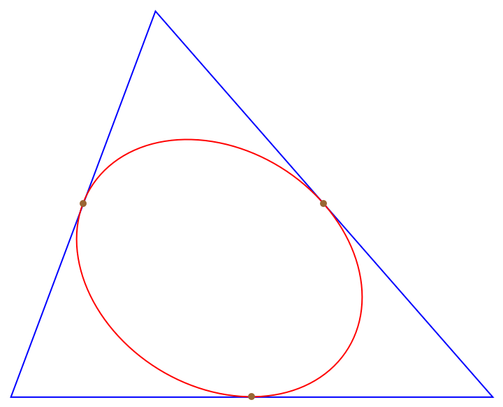 |
This work is licensed under a Creative Commons Attribution 4.0 International License
![p[z_] := (24 + 7 I) - 25 z - 7 I z^2 + z^3;
rts = z /. Solve[p[z] == 0, z]; Graphics[{FaceForm[], {EdgeForm[ColorData[97, 4]], Triangle[ReIm[rts]]}, {AbsolutePointSize[5], ColorData[97, 4], Point[ReIm[rts]]}, {EdgeForm[ColorData[97, 3]], TransformedRegion[
ResourceFunction["SteinerCircumellipse"][ReIm[rts]], ScalingTransform[{1/2, 1/2}, ReIm[Mean[rts]]]]}, {AbsolutePointSize[4], ColorData[97, 3], Point[ReIm[z /. Solve[p'[z] == 0, z]]]}}]](https://www.wolframcloud.com/obj/resourcesystem/images/cf0/cf01e293-cf19-4344-b7b1-bf0bb605974b/224df2154e069e3b.png)