Basic Examples (5)
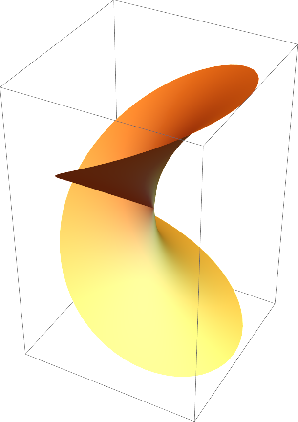
The Riemann surface of the square root functions plotted as the real part of  :
:
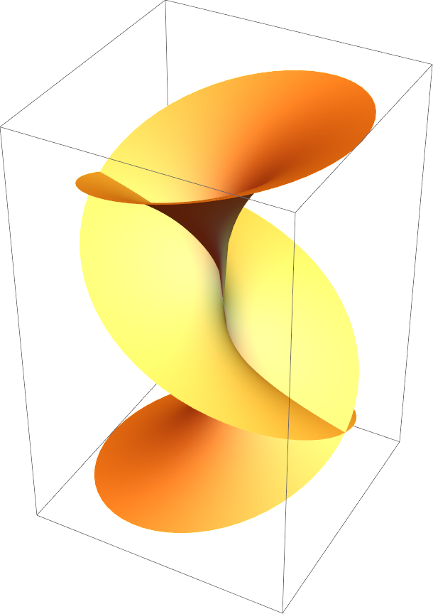
The Riemann surface of the cube root functions plotted as the real part of  :
:
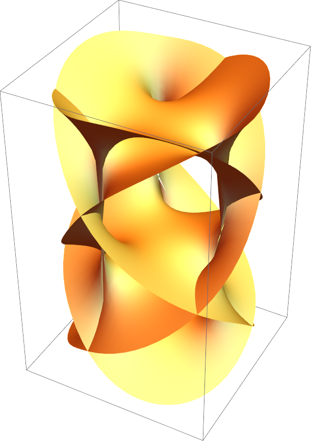
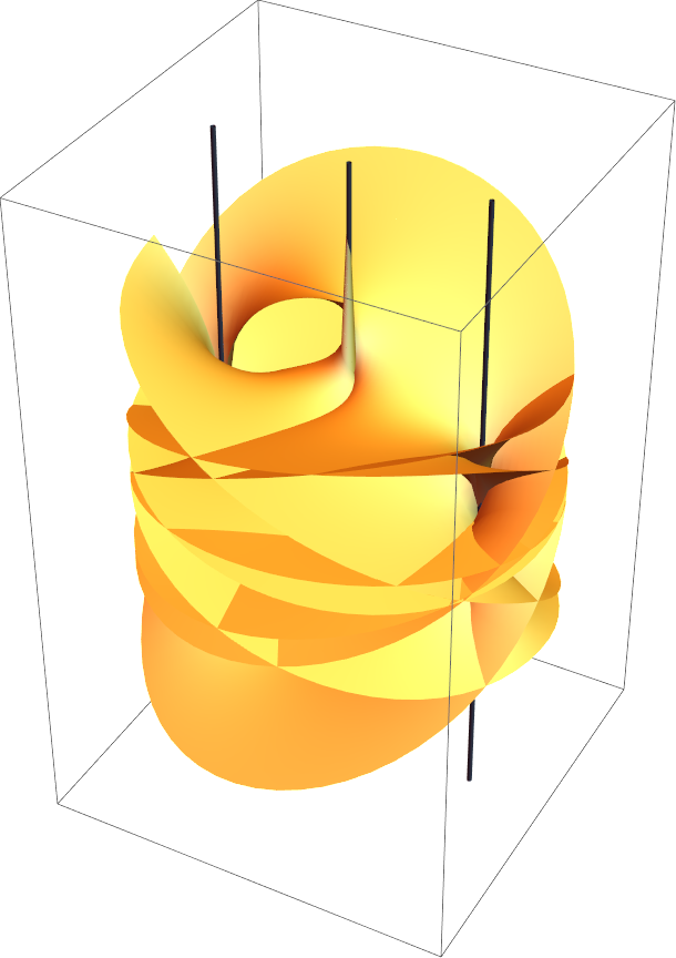
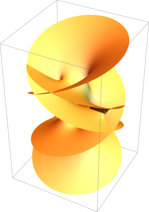
The Riemann surface of the function w defined implicitly through w5=1-z3:
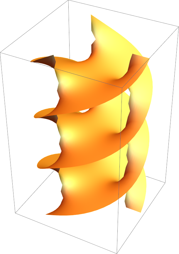
The Riemann surface of a function with three logarithmic branch points at z=1, z=-(-1)1/3, and z=-(-1)2/3:
The Riemann surface of a more complicated function with multiple logarithmic branch points:
Scope (6)
The (vertical) function value displayed can be any linear combination of Re(z), Im(z), Re(w), Im(w):
The {x,y,z}-values displayed can be any linear combination of Re(z), Im(z), Re(w), Im(w):
A wide class of compositions of elementary functions can be visualized. Here are some examples containing trigonometric and inverse trigonometric functions:
Riemann surface of nested square and cube roots:
Root objects define implicitly bivariate polynomials and the corresponding Riemann surface can be plotted. Here is an irreducible quantic shown:
For the purpose of the RiemannSurfacePlot3D function, the product log function is considered an elementary function:
Here are the real and imaginary parts of the function  :
:
The vertical value of the surface can be a linear combination of the real and imaginary parts of z and w:
Even all three coordinate values of the surface can be such a linear combination:
Options (17)
PlotStyle (2)
Specify a plot style for the whole Riemann surface:
A list of style directives will be applied cyclically to the radial-azimuthal patches that result from the branch point-induced tensor-product subdivision of the complex z-plane:
ColorFunction (3)
Color the surface according to the argument of w:
Use a color functions that depends on  :
:
Color a Riemann surface according to the distance to the nearest branch point, with parts of the surface that are near to a branch point being red:
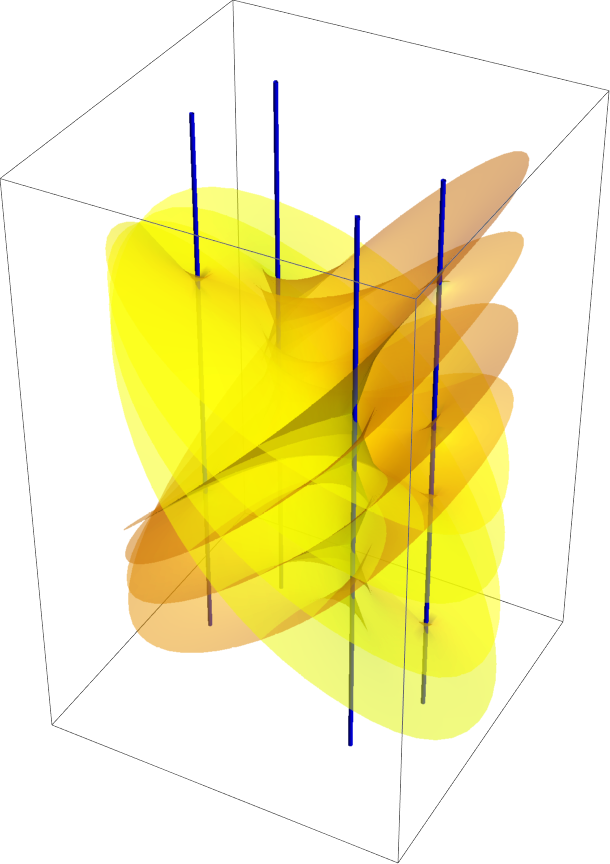
ShowBranchPoints and BranchPointStyle (2)
With the setting "ShowBranchPoints"→True, branch points over the z-plane will be indicated as vertical tubes (mouseover the vertical tubes to see z-positions of the branch points):
The option "BranchPointStyle" determines the color of these tubes:
BranchPointPlotRangeFactor (2)
The default plot range extends the distance from the origin to the furthest branch point by 50%:
Show the Riemann surface with more padding (but same box ratios):
LogSheets (1)
Logarithmic branch points connect infinitely many sheets. By default, the principal sheet and one sheet below and above are used. Using the option "LogSheets", more or fewer sheets could be displayed:
BranchPointOffset (2)
The default the numerical computation of the surface patches starts 10-6 away from any branch point. For most surfaces this results in defacto invisible gaps between the patches:
By specifying a larger offset from the branch point-generated patches gaps between the patches become visible. The next input colors the patches differently:
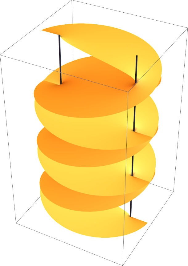
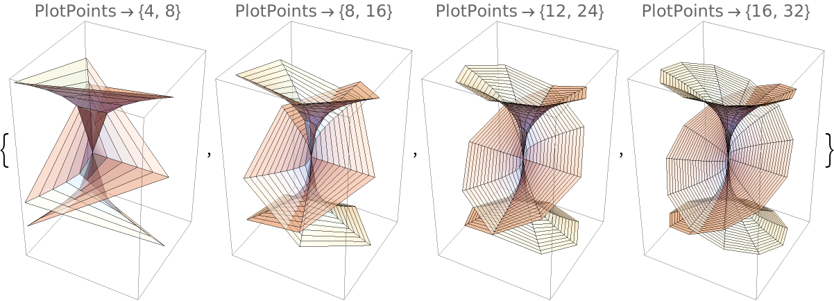
PlotPoints (1)
The option PlotPoints determines the approximate number of radial and azimuthal plot points:
StitchPatches (2)
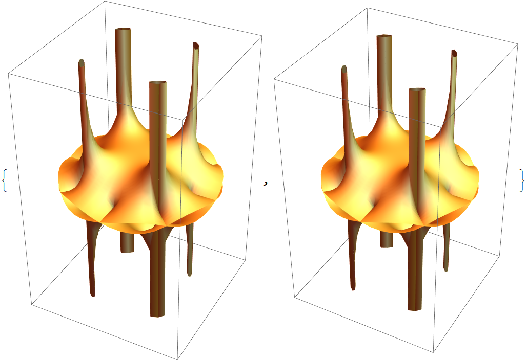
The option "StitchPatches" tries to connect neighboring patches by stitching them together with tiny polygons to obtain water-tight surfaces:
While visually the two graphics are quite similar, the stitched patches result in a larger number of graphics complexes in the resulting 3D graphic:
Graphics3D options (2)
All options of Graphics3D can be specified:
Plot of the Riemann surface of a general quartic polynomial with multiple options specified:
Applications (5)
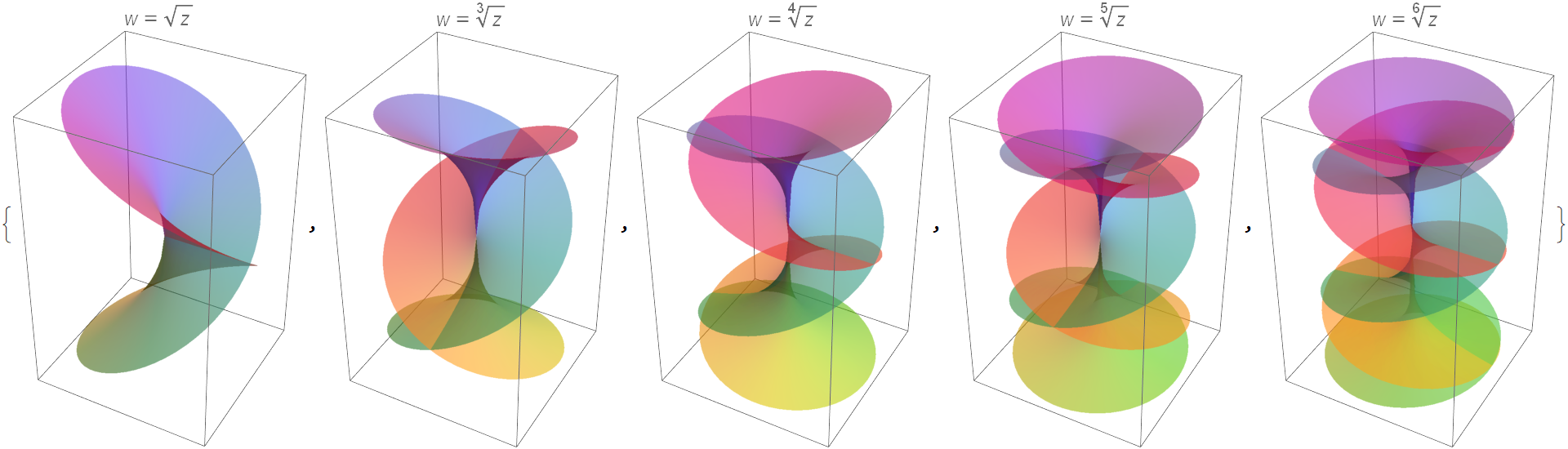
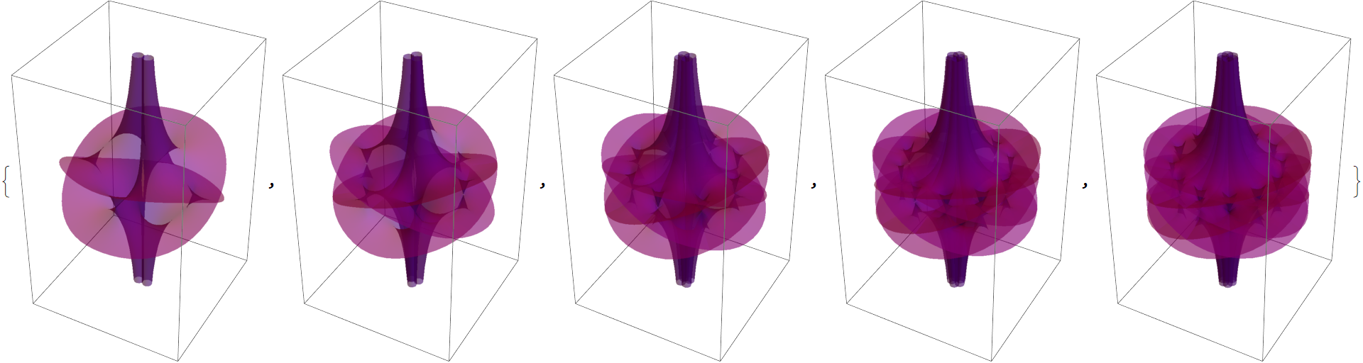
Show the Riemann surfaces for the simple power functions  colored by the argument of w:
Replacing z→zn+z-n in the last example gives more complicated surfaces with a pole at z=0:
Riemann surfaces of general cubics (in total degree) polynomials might or might not have poles:
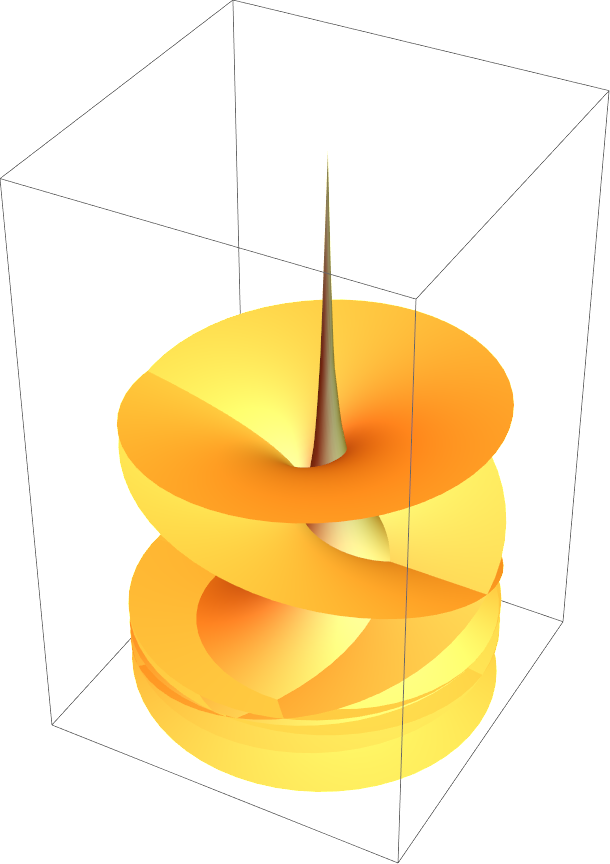
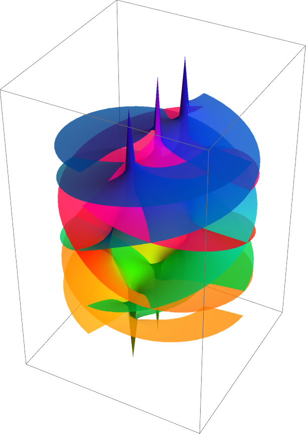
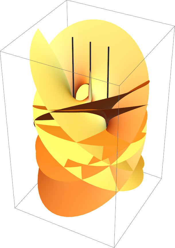
Real parts of logarithms typically show (logarithmic) singularities, visible as long thin tubes extending up or down. Imaginary parts often are bounded.:
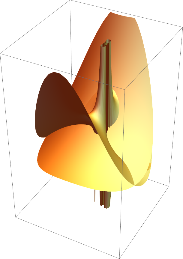
Logarithmic and algebraic branch points can be at the same z-values:
Properties and Relations (10)
Inverse trigonometric functions can be expressed through logarithms and so the Riemann surfaces of such functions show logarithmic branch points:
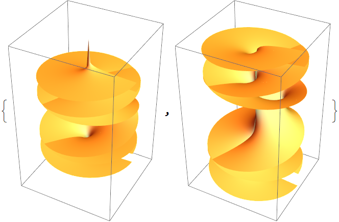
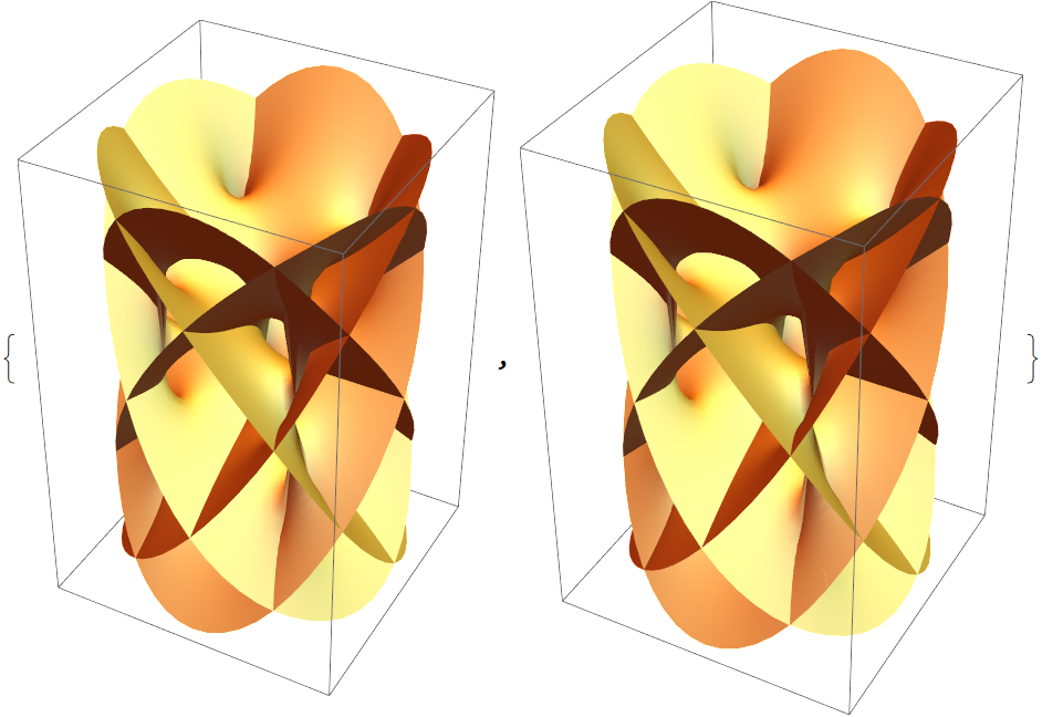
Two Riemann surfaces of functions containing square roots and logarithms:
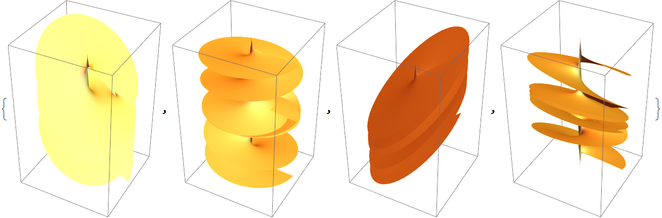
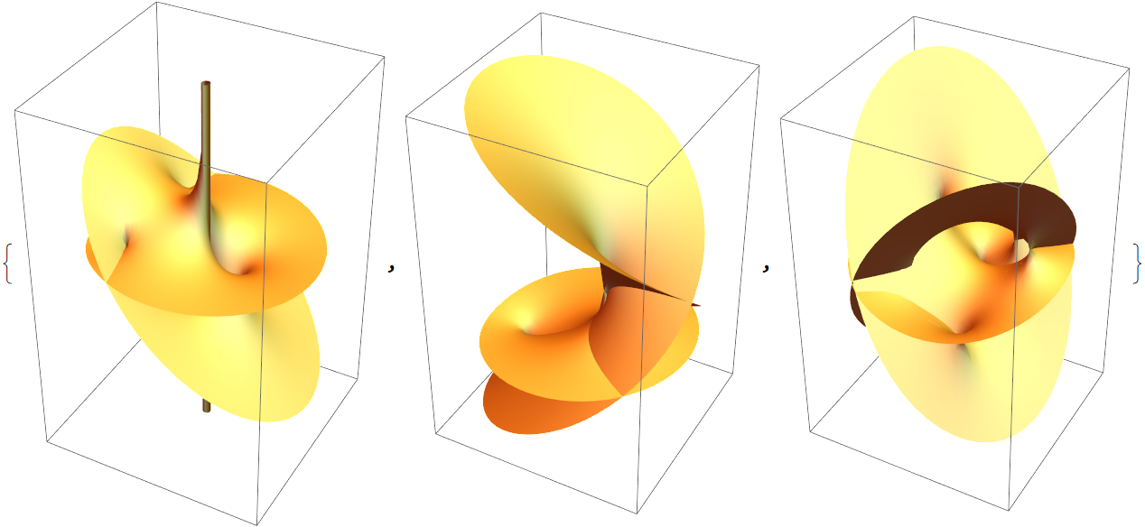
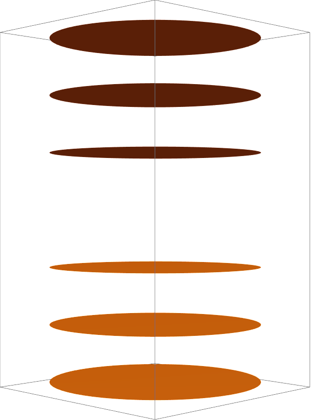
When displaying the real or imaginary part vertically, Riemann surfaces can potentially separate into disconnected parts:
Linear combinations of Re(w) and Im(w) typically result in connected Riemann surfaces:
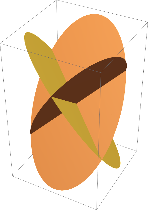
The Riemann surface of  also splits into separate (intersecting, but not smoothly connected) pieces:
The Riemann surface of  also splits into separate pieces:
Note that the classic identity  holds only for positive real z:
Expressions containing square roots and logarithms that become equal after PowerExpand are often not equivalent for all complex numbers. Here is an example:
But the Riemann surfaces of such expressions are identical:
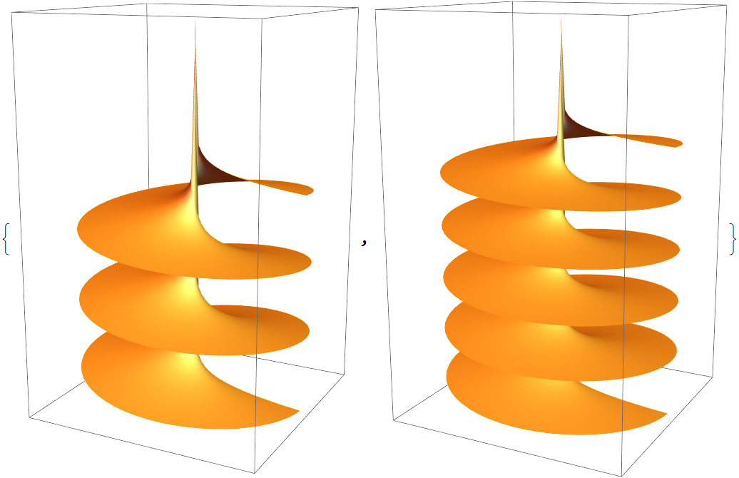
In the following example, asymptotically  approaches a constant. The cube root shows the three values of the constant:
Using a logarithm instead shows a Riemann surface with infinitely many sheets (we display 5=4+1/2+1/2):
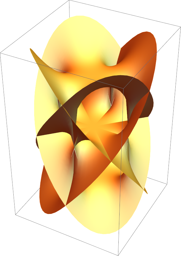
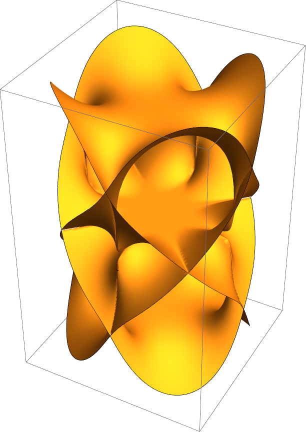
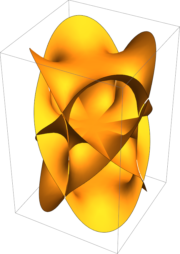
The Riemann surface of roots of polynomials displayed as the real and imaginary part are typically visually quite similar (note the slightly different orientation):
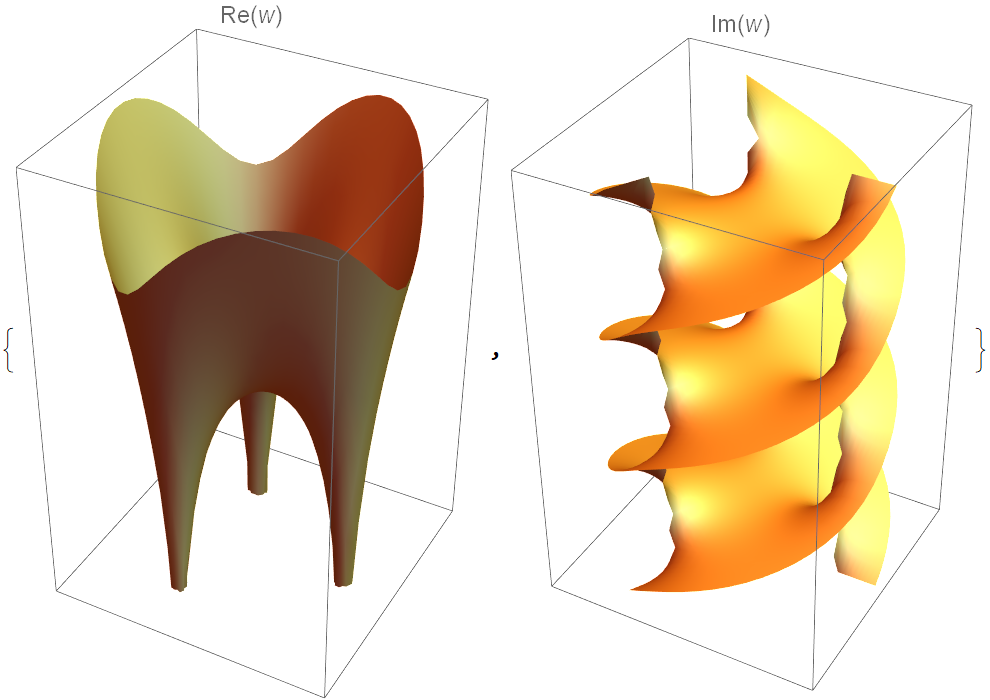
For functions containing logarithms, the real and imaginary parts typically look quite different:
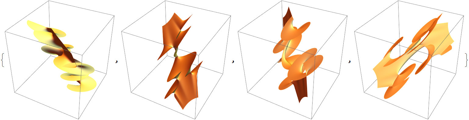
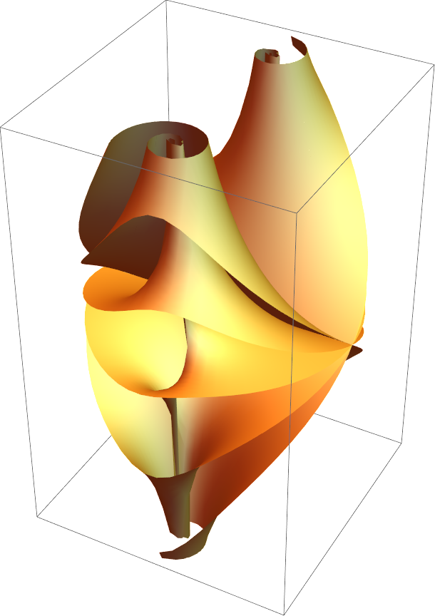
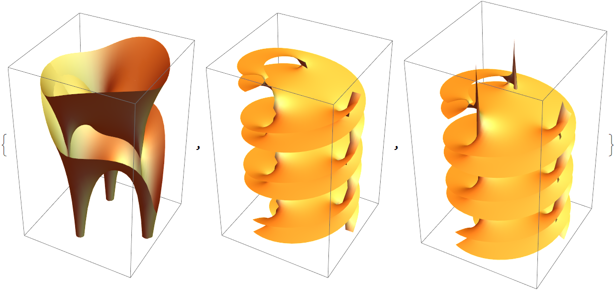
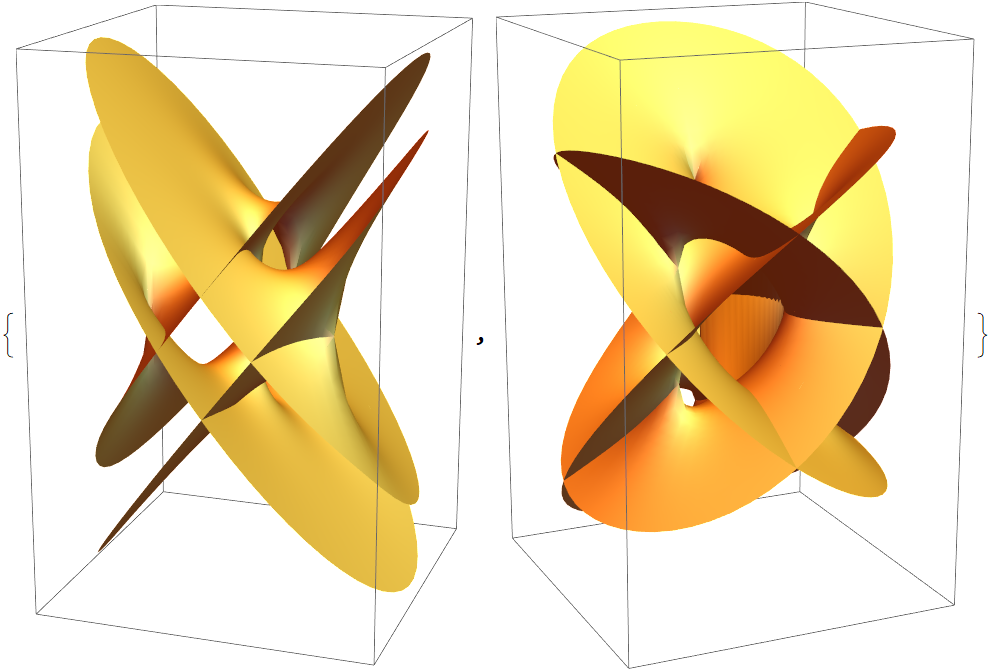
Riemann surfaces constructed from nested radicals can take on a large variety of shapes:
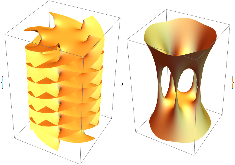
Compare the result of RiemannSurfacePlot3D with two other construction methods for Riemann surfaces:
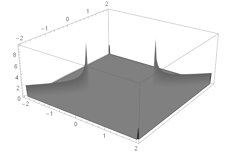
For Riemann surfaces defined through bivariate polynomials one can separate the real and imaginary parts and eliminate variables. The next inputs computes an implicit form of v=Im(w) as a functions of x=Re(z) and y=Im(z) for w3=1-z4:
The implicit form is a total degree 16 trivariate polynomial:
Using ContourPlot3D we obtain the following surface:
Alternatively one can use Plot3D to plot every sheet and then show all sheets (note the gaps that arise from the Exclusions option of Plot3D):
Possible Issues (2)
Only multi-valued functions are plotted:
Even simple-looking functions with multiple logarithmic branch points can generates plots with many sheets:
Neat Examples (18)
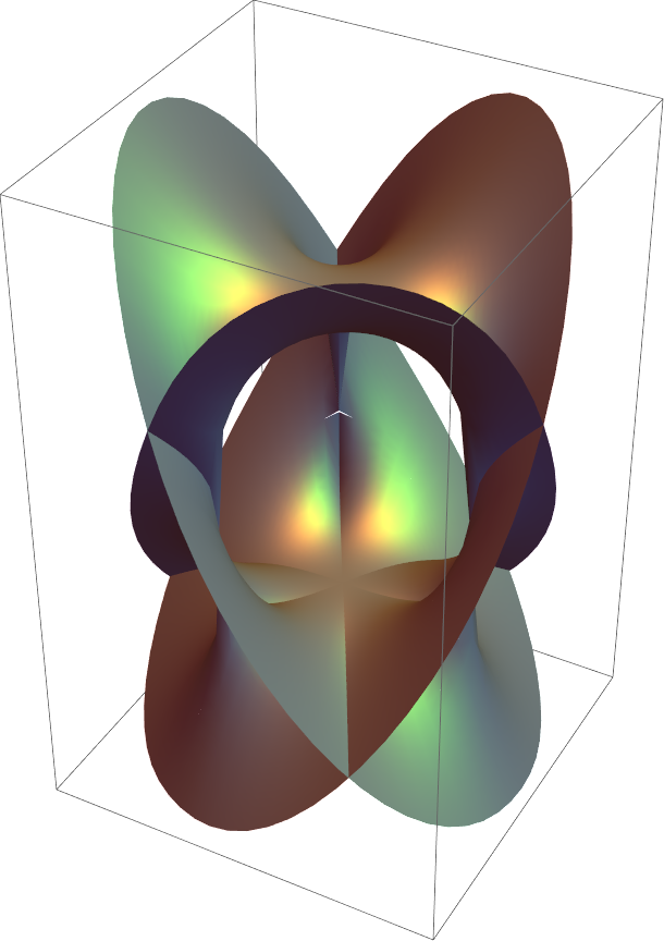
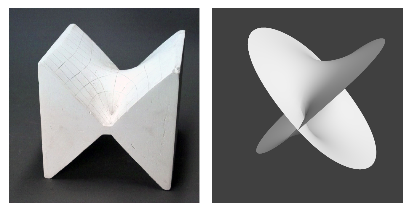
Compare the Riemann surface  with the plaster model (left) from Schilling's catalog (image from the Göttingen Collection of Mathematical Models and Instruments) with the plot from RiemannSurfacePlot3D (right):
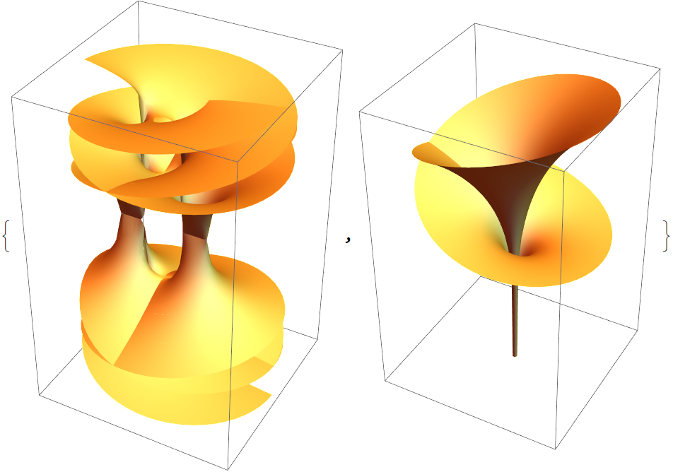
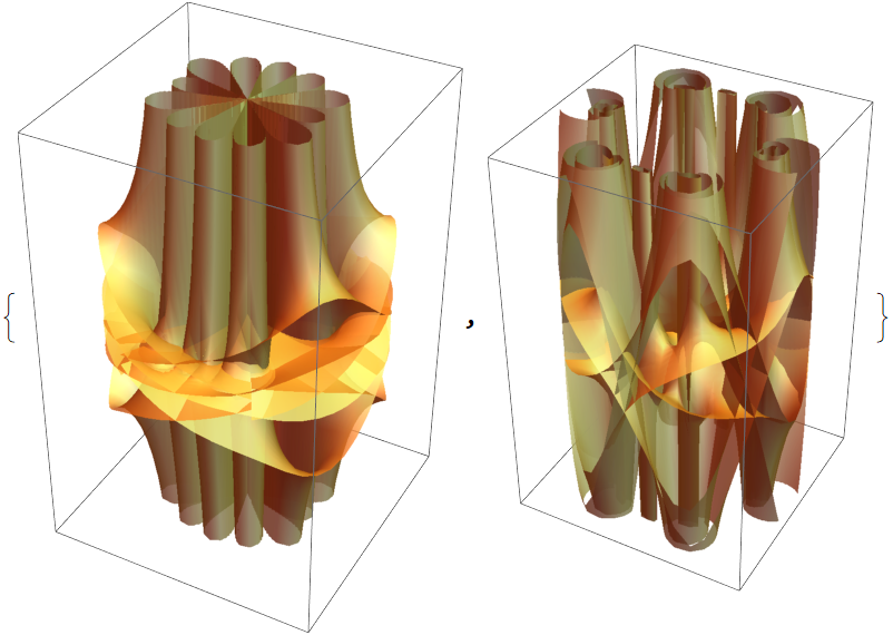
Two Riemann surfaces of quotients of square roots and logarithms:
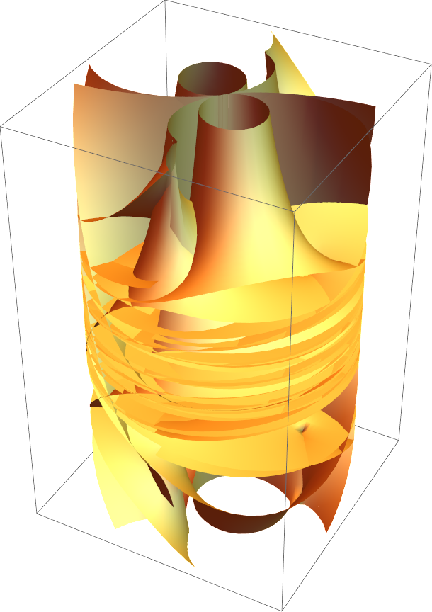
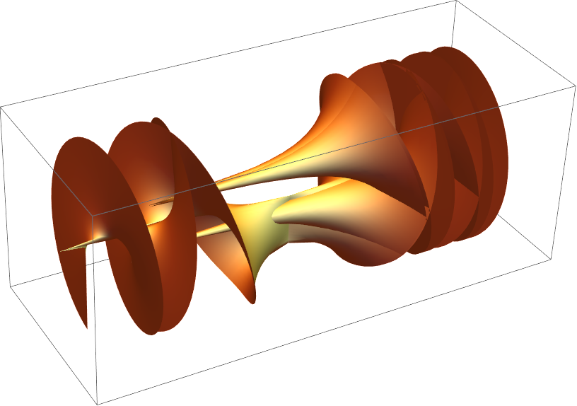
The rotated (for a more interesting look) Riemann surface of  :
:
The rotated (for a more interesting look) Riemann surface of  :
:
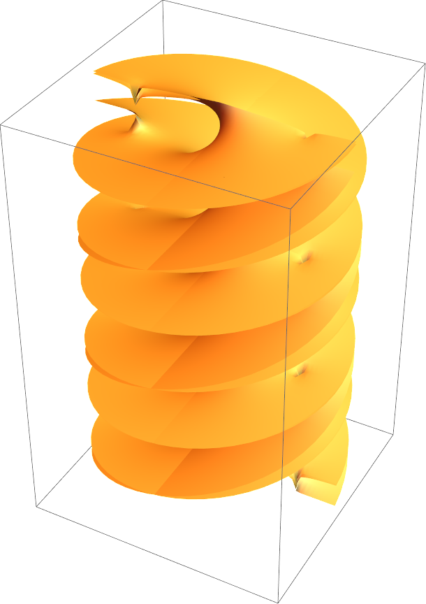
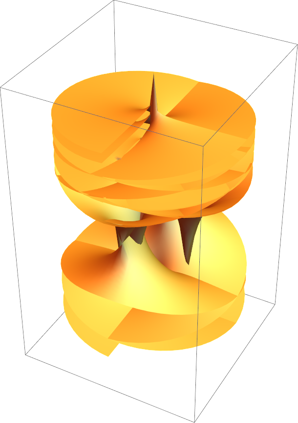
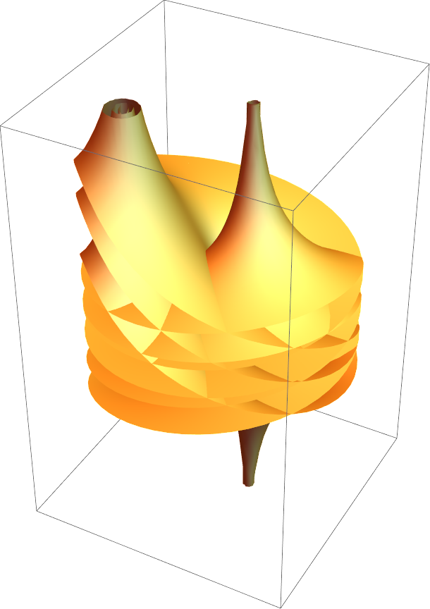
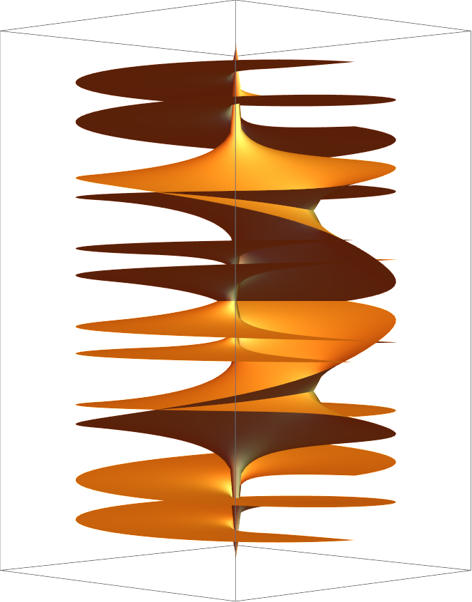
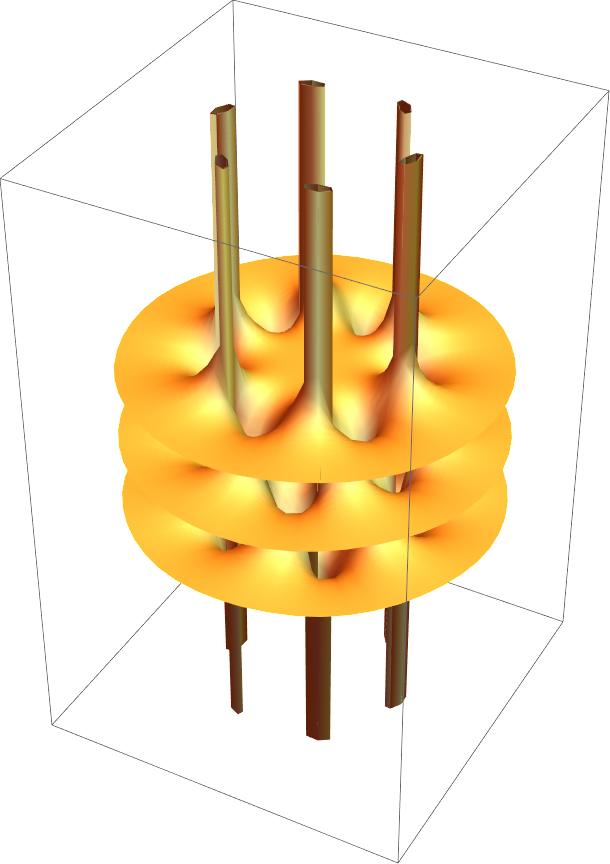
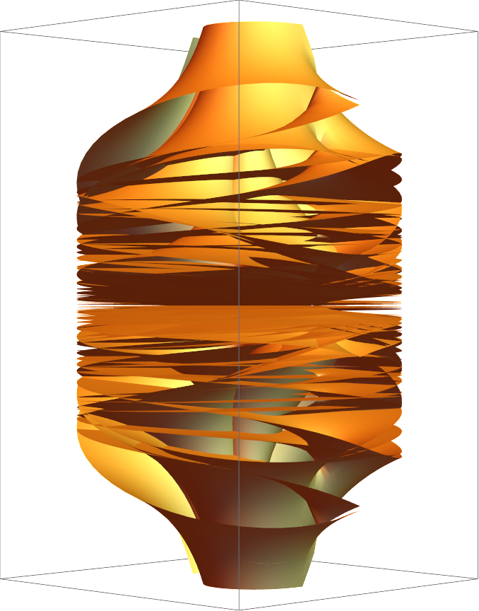
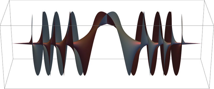
The imaginary parts of of the Riemann surface of  reminds of nested tops:
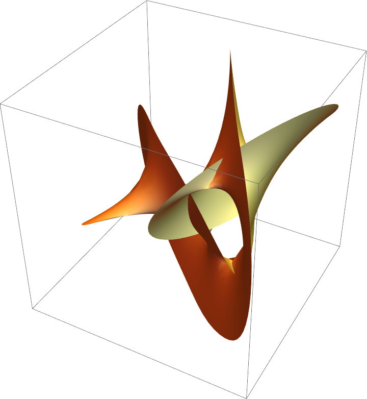
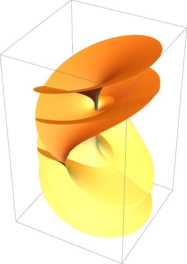
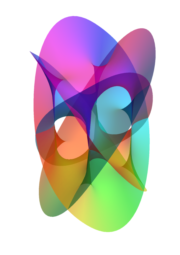
The Riemann surface of  colored according to the argument of w:
Color the real part according to the imaginary part:
Color the sheets according to the argument of the z-value:
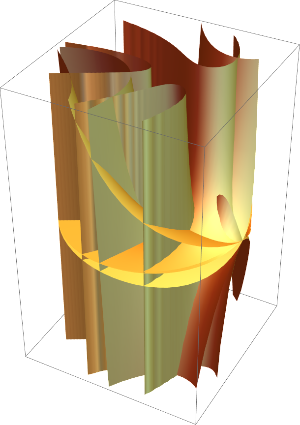
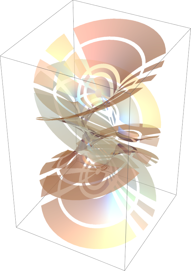
The internals of this Riemann surface of a ratio of arctan functions:
Color the surface blue when the real part of w is greater than the imaginary part, red otherwise:
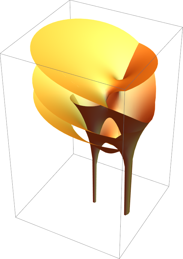
The complicated Riemann surface of the square root of the logarithm of a polynomial:
Plot a camouflaged Riemann surface:
Plot a simple Riemann surface:
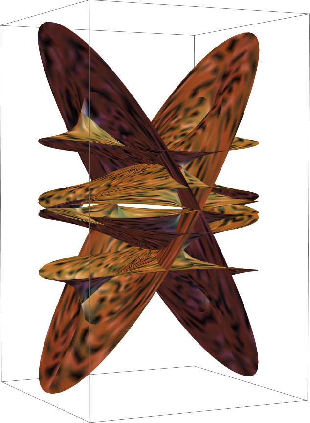
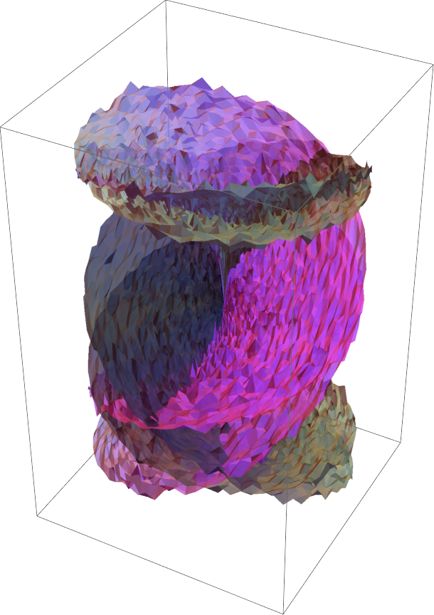
"Roughen" the Riemann surface by moving of the surface by small random amounts:
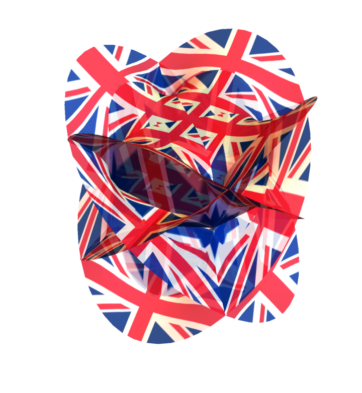
Add the Union Jack into the patches of a Riemann surface as a texture:
A Riemann surface that slowly fades out:
Plot an auto-rotating Riemann surface:
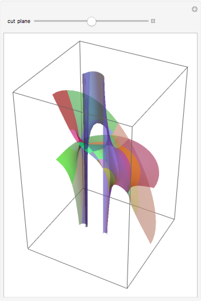
Cut a Riemann surface along shifted x-, y-planes:
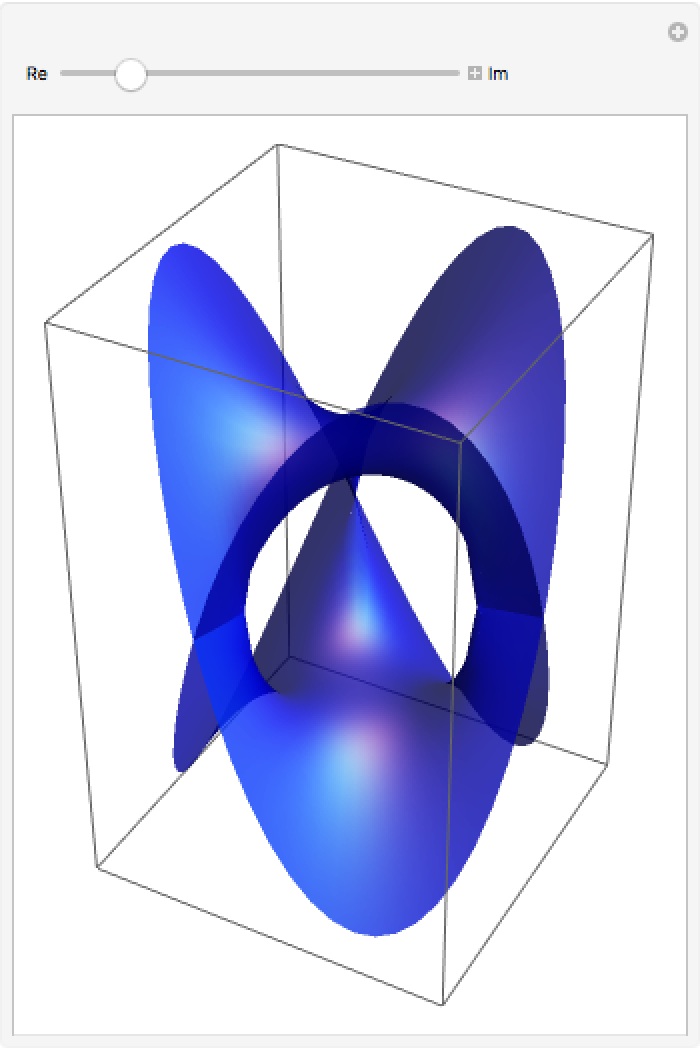
Smoothly change from displaying the real part to displaying the imaginary parts of  :
:
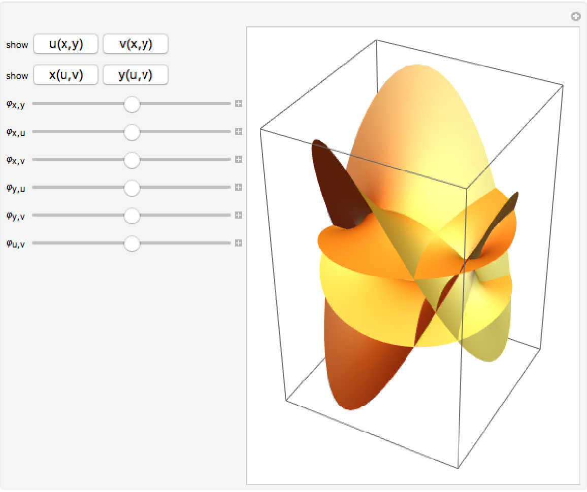
By considering a Riemann surface as part of  , by rotating the surface and projecting into 2D space one can interactively explore the complete Riemann surface. Every angle results in a different 3D surface:
![ResourceFunction["RiemannSurfacePlot3D"][
w == Sqrt[z^2 + 1] + Sqrt[z - 1], Re[w] + 2 Im[w] - Re[z]/5, {z, w}, ViewPoint -> {-3.08, -1.41, -0.0}]](https://www.wolframcloud.com/obj/resourcesystem/images/540/5409a3e7-a791-40b6-9f12-75d6be8fa109/4c3f846bd97b2dc6.png)

![ResourceFunction["RiemannSurfacePlot3D"][
w == Sqrt[z^2 - I] + Sqrt[z - 1], {Re[z] + Im[w], Im[z] + Re[w], Re[w] + Im[w] - Re[z]}, {z, w}]](https://www.wolframcloud.com/obj/resourcesystem/images/540/5409a3e7-a791-40b6-9f12-75d6be8fa109/739ce689f668f5c8.png)

![{ResourceFunction["RiemannSurfacePlot3D"][w == Sqrt[I - Log[z]], Re[w], {z, w}],
ResourceFunction["RiemannSurfacePlot3D"][w == Sqrt[I - Log[z]], Im[w], {z, w}]}](https://www.wolframcloud.com/obj/resourcesystem/images/540/5409a3e7-a791-40b6-9f12-75d6be8fa109/3605cb4a58b29e5f.png)
![Table[ResourceFunction["RiemannSurfacePlot3D"][w == Sqrt[I - Log[z]], RandomReal[{-1, 1}, 4] . {Re[z], Im[z], Re[w], Im[w]}, {z, w}], {4}]](https://www.wolframcloud.com/obj/resourcesystem/images/540/5409a3e7-a791-40b6-9f12-75d6be8fa109/61e5828dfa80f558.png)
![Table[ResourceFunction["RiemannSurfacePlot3D"][w == Sqrt[I - Log[z]], Table[RandomReal[{-1, 1}, 4] . {Re[z], Im[z], Re[w], Im[w]}, 3], {z,
w}], {4}]](https://www.wolframcloud.com/obj/resourcesystem/images/540/5409a3e7-a791-40b6-9f12-75d6be8fa109/3690d7163607225c.png)
![ResourceFunction["RiemannSurfacePlot3D"][w == Power[1 - z^3, (3)^-1], Re[w], {z, w}, PlotStyle -> Directive[GrayLevel[0.5], Specularity[Yellow, 20]]]](https://www.wolframcloud.com/obj/resourcesystem/images/540/5409a3e7-a791-40b6-9f12-75d6be8fa109/4b5806362488cb4d.png)
![ResourceFunction["RiemannSurfacePlot3D"][w == Power[1 - z^3, (3)^-1], Re[w], {z, w}, PlotStyle -> Table[Directive[Opacity[0.5], RandomColor[]], {25}]]](https://www.wolframcloud.com/obj/resourcesystem/images/540/5409a3e7-a791-40b6-9f12-75d6be8fa109/45af21e095864066.png)
![ResourceFunction["RiemannSurfacePlot3D"][w == Sqrt[Log[z + z^3]], Im[w], {z, w}, ColorFunction -> (Directive[Opacity[0.8], Hue[(Arg[#2] + Pi)/(2 Pi)]] &)]](https://www.wolframcloud.com/obj/resourcesystem/images/540/5409a3e7-a791-40b6-9f12-75d6be8fa109/6a8c2218b2e8e0f9.png)
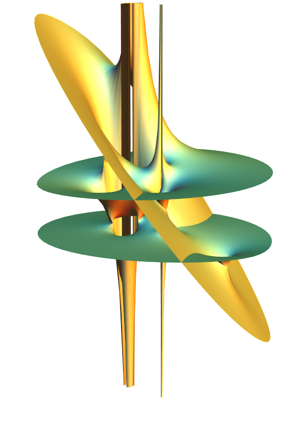
![ResourceFunction["RiemannSurfacePlot3D"][w == Sqrt[z/Log[z]], Im[w], {z, w}, ColorFunction -> (Directive[Opacity[0.5], ColorData["GreenPinkTones"][(ArcTan[Abs[#1] + Abs[#2]] + 1)/
2]] &)]](https://www.wolframcloud.com/obj/resourcesystem/images/540/5409a3e7-a791-40b6-9f12-75d6be8fa109/58052c94a6fe8ec4.png)
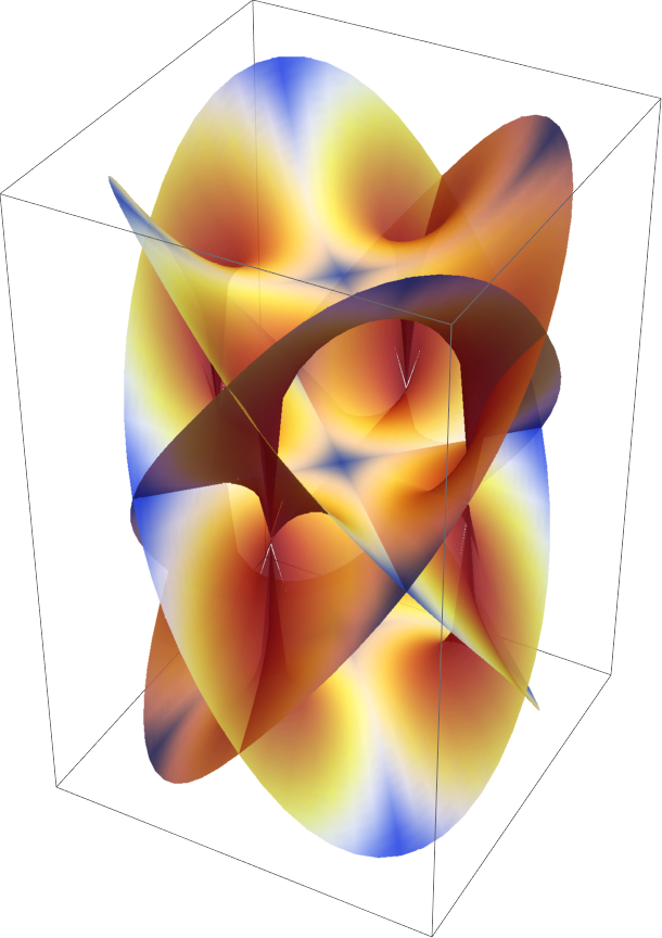
![ResourceFunction["RiemannSurfacePlot3D"][w == Power[1 - z^4, (4)^-1], Im[w], {z, w}, ColorFunction -> (Directive[Opacity[0.9], ColorData["TemperatureMap"][
1 - Min[Function[bc, Abs[#1 - bc]] /@ {1, -1, I, -I}]^2]] &)]](https://www.wolframcloud.com/obj/resourcesystem/images/540/5409a3e7-a791-40b6-9f12-75d6be8fa109/744797cd421dadd4.png)
![ResourceFunction["RiemannSurfacePlot3D"][
w == Sqrt[z - 1] + Sqrt[z + 1] - 2 Sqrt[z^2 + I], Re[w], {z, w}, PlotStyle -> Directive[Opacity[0.5], Yellow], "ShowBranchPoints" -> True, "BranchPointStyle" -> Blue]](https://www.wolframcloud.com/obj/resourcesystem/images/540/5409a3e7-a791-40b6-9f12-75d6be8fa109/4d38fdb57eaf736f.png)
![{ResourceFunction["RiemannSurfacePlot3D"][w == -Log[z], Re[w] + Im[w], {z, w}, ViewPoint -> {1.1, -2.15, 0.6}],
ResourceFunction["RiemannSurfacePlot3D"][w == -Log[z], Re[w] + Im[w], {z, w}, "LogSheets" -> {-2, -1, 0, 1, 2}, ViewPoint -> {1.1, -2.15, 0.6}]}](https://www.wolframcloud.com/obj/resourcesystem/images/540/5409a3e7-a791-40b6-9f12-75d6be8fa109/2e7be1013fca3f39.png)
![ResourceFunction["RiemannSurfacePlot3D"][
w == Root[1 - z^2 + 2 z #^2 + #^5 &, 1], Im[w], {z, w},
"BranchPointOffset" -> 0.08, PlotStyle -> Table[Directive[Opacity[RandomReal[{0.8, 0.9}]], GrayLevel[0.7], Specularity[ColorData["TemperatureMap"][RandomReal[]], 20]], {100}]]](https://www.wolframcloud.com/obj/resourcesystem/images/540/5409a3e7-a791-40b6-9f12-75d6be8fa109/3c99158f75aad7ed.png)
![Table[ResourceFunction["RiemannSurfacePlot3D"][w == z^(1/3), Im[w], {z, w}, PlotPoints -> j {3, 6}, PlotLabel -> (PlotPoints -> j {4, 8}), PlotStyle -> Directive[Opacity[0.6], EdgeForm[{Thickness[0.001], Black}]]], {j, 4}]](https://www.wolframcloud.com/obj/resourcesystem/images/540/5409a3e7-a791-40b6-9f12-75d6be8fa109/24e93802f4447aab.png)
![{ResourceFunction["RiemannSurfacePlot3D"][w == (z^2 + z^6)^(1/6), Im[w], {z, w}],
ResourceFunction["RiemannSurfacePlot3D"][w == (z^2 + z^6)^(1/6), Im[w], {z, w}, "StitchPatches" -> True]}](https://www.wolframcloud.com/obj/resourcesystem/images/540/5409a3e7-a791-40b6-9f12-75d6be8fa109/7be7fb5aea01ad9b.png)
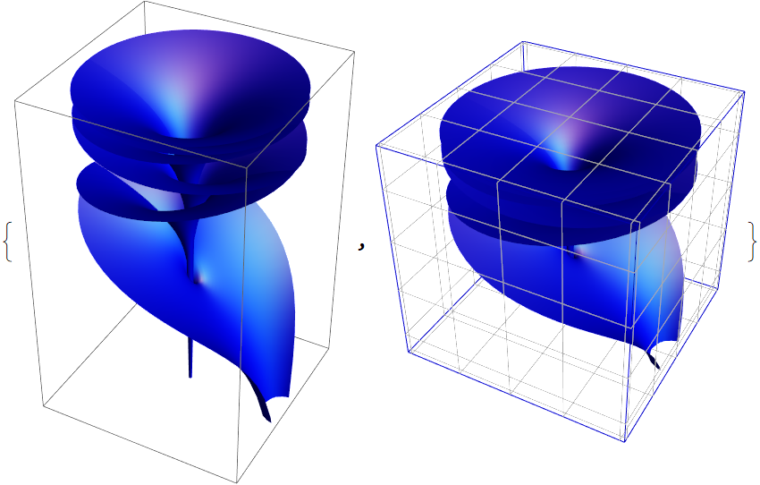
![{ResourceFunction["RiemannSurfacePlot3D"][
w == Log[Sqrt[z] + Power[z, (3)^-1]], Re[w], {z, w}, PlotStyle -> Directive[Blue, Specularity[Yellow, 12]]],
ResourceFunction["RiemannSurfacePlot3D"][
w == Log[Sqrt[z] + Power[z, (3)^-1]], Re[w], {z, w},
PlotStyle -> Directive[Blue, Specularity[Yellow, 12]], BoxRatios -> {1, 1, 1}, FaceGrids -> All, BoxStyle -> Darker[Blue]]}](https://www.wolframcloud.com/obj/resourcesystem/images/540/5409a3e7-a791-40b6-9f12-75d6be8fa109/2e972cc878a166ef.png)
![ResourceFunction[
"RiemannSurfacePlot3D"][-1 + z (-(1 + I) z^2 + z - 1) - w (1 + (z - 1) z (z - I)) + I w^2 ( (z - 1) z^2 - 1) - (z ((1 + I) + z) - I) w^3 == 0, Re[w], {z, w}, PlotRange -> 6.5 {-1, 1}, ViewPoint -> {3.3, 0.49, 0.6}, PlotStyle -> Directive[Specularity[GrayLevel[1], 3], RGBColor[
0.880722, 0.611041, 0.142051]], Boxed -> False,
Lighting -> {{"Ambient", Hue[0.65, 0.6, 0.6]}, {"Directional", RGBColor[0.7, 0, 0], ImageScaled[{3, 0, 2}]}, {"Directional", RGBColor[0, 0.7, 0], ImageScaled[{1.5`, 1.5`, 2}]}, {"Directional", RGBColor[
0, 0, 0.7], ImageScaled[{0, 3, 2}]}}]](https://www.wolframcloud.com/obj/resourcesystem/images/540/5409a3e7-a791-40b6-9f12-75d6be8fa109/20687ba3a8c1de9b.png)
![Table[ResourceFunction["RiemannSurfacePlot3D"][w == z^(1/n), Im[w], {z, w},
ImageSize -> 180, PlotLabel -> w == z^(1/n), ColorFunction -> (Directive[Opacity[0.6], ColorData["BalancedHue"][(Arg[#2] + Pi)/(2 Pi)]] &)],
{n, 2, 6}]](https://www.wolframcloud.com/obj/resourcesystem/images/540/5409a3e7-a791-40b6-9f12-75d6be8fa109/281b90c51600ed4b.png)
![Table[ResourceFunction["RiemannSurfacePlot3D"][
w == Power[z^n - 1/z^n, (n)^-1], Im[w], {z, w}, ImageSize -> 180, PlotStyle -> Directive[Opacity[0.6], Purple]],
{n, 2, 6}]](https://www.wolframcloud.com/obj/resourcesystem/images/540/5409a3e7-a791-40b6-9f12-75d6be8fa109/0dc5ef7173093e4f.png)
![(* Evaluate this cell to get the example input *) CloudGet["https://www.wolframcloud.com/obj/a18f486b-4dad-4d28-b5d5-b588426ea87e"]](https://www.wolframcloud.com/obj/resourcesystem/images/540/5409a3e7-a791-40b6-9f12-75d6be8fa109/667cb12daf6a103c.png)
![{ResourceFunction["RiemannSurfacePlot3D"][w == Log[z^3 - 1], Re[w], {z, w}, PlotLabel -> Re[w]],
ResourceFunction["RiemannSurfacePlot3D"][w == Log[z^3 - 1], Im[w], {z, w}, PlotLabel -> Im[w]]}](https://www.wolframcloud.com/obj/resourcesystem/images/540/5409a3e7-a791-40b6-9f12-75d6be8fa109/098480a2f6761b05.png)
![{ResourceFunction["RiemannSurfacePlot3D"][w == Log[z] + Sqrt[z], Im[w], {z, w}, "ShowBranchPoints" -> True],
ResourceFunction["RiemannSurfacePlot3D"][w == Log[z] * Sqrt[z], Re[w], {z, w}, "ShowBranchPoints" -> True]}](https://www.wolframcloud.com/obj/resourcesystem/images/540/5409a3e7-a791-40b6-9f12-75d6be8fa109/7143233a280e4205.png)

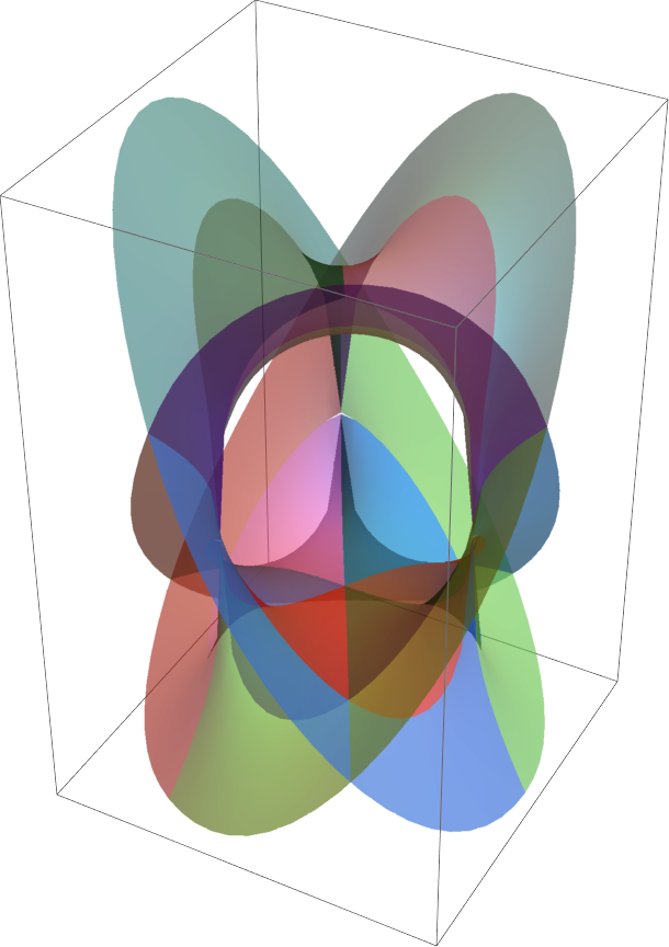
![{ResourceFunction["RiemannSurfacePlot3D"][w == ArcSin[Sqrt[z^5 - 1]], Re[w], {z, w}],
ResourceFunction["RiemannSurfacePlot3D"][w == ArcSin[Sqrt[z^5 - 1]],
Im[w], {z, w}]}](https://www.wolframcloud.com/obj/resourcesystem/images/540/5409a3e7-a791-40b6-9f12-75d6be8fa109/25dfc622af9d2276.png)
![{ResourceFunction["RiemannSurfacePlot3D"][w == Sqrt[Log[z + z^2]], Re[w], {z, w}],
ResourceFunction["RiemannSurfacePlot3D"][w == -2 Sqrt[z] + Log[z], Re[w], {z, w}]}](https://www.wolframcloud.com/obj/resourcesystem/images/540/5409a3e7-a791-40b6-9f12-75d6be8fa109/4ab321827ddc3f33.png)
![{ResourceFunction["RiemannSurfacePlot3D"][w == Sqrt[1 + Sqrt[Log[z]]],
Re[w], {z, w}, ViewPoint -> {3, -3, 1.5}],
ResourceFunction["RiemannSurfacePlot3D"][w == Sqrt[1 + Sqrt[Log[z]]],
Im[w], {z, w}, ViewPoint -> {3, -3, 1.5}]}](https://www.wolframcloud.com/obj/resourcesystem/images/540/5409a3e7-a791-40b6-9f12-75d6be8fa109/4ba2a3d4a8a070d0.png)
![ComplexPlot3D[
Sqrt[(1 - z^4)/(1 + z^4)] - Sqrt[1 - z^4]/
Sqrt[1 + z^4], {z, -2 - 2 I, 2 + 2 I}, Exclusions -> {}, PlotRange -> All, ColorFunction -> (Gray &)]](https://www.wolframcloud.com/obj/resourcesystem/images/540/5409a3e7-a791-40b6-9f12-75d6be8fa109/060b9b7c55879092.png)
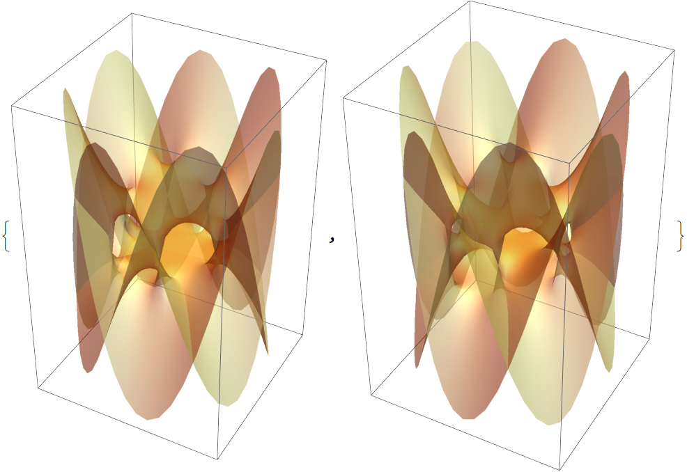
![{ResourceFunction["RiemannSurfacePlot3D"][
w == Sqrt[1 - z^4]/Sqrt[1 + z^4], Re[w], {z, w}],
ResourceFunction["RiemannSurfacePlot3D"][
w == Sqrt[(1 - z^4)/(1 + z^4)], Re[w], {z, w}]}](https://www.wolframcloud.com/obj/resourcesystem/images/540/5409a3e7-a791-40b6-9f12-75d6be8fa109/030c6e39ed1c8910.png)
![ResourceFunction["RiemannSurfacePlot3D"][
w == Power[(1 + z^6)/(1 - z^6), (3)^-1], Im[w], {z, w}, BranchPointPlotRangeFactor -> 2]](https://www.wolframcloud.com/obj/resourcesystem/images/540/5409a3e7-a791-40b6-9f12-75d6be8fa109/50e8190b5355395a.png)
![ResourceFunction["RiemannSurfacePlot3D"][
w == Log[(1 + z^6)/(1 - z^6)], Im[w], {z, w}, "BranchPointPlotRangeFactor" -> 2, "LogSheets" -> {-2, -1, 0, 1, 2}]](https://www.wolframcloud.com/obj/resourcesystem/images/540/5409a3e7-a791-40b6-9f12-75d6be8fa109/537809b08105bb62.png)
![{ResourceFunction["RiemannSurfacePlot3D"][
w == Power[8 - 3 z - 2 z^4 + z^7, (3)^-1], Re[w], {z, w}, PlotStyle -> Opacity[0.6]],
ResourceFunction["RiemannSurfacePlot3D"][
w == Power[8 - 3 z - 2 z^4 + z^7, (3)^-1], Im[w], {z, w}, PlotStyle -> Opacity[0.6]]}](https://www.wolframcloud.com/obj/resourcesystem/images/540/5409a3e7-a791-40b6-9f12-75d6be8fa109/761f2165e136b2b0.png)
![(* Evaluate this cell to get the example input *) CloudGet["https://www.wolframcloud.com/obj/607eb47d-73f5-480f-963e-62dc11965f93"]](https://www.wolframcloud.com/obj/resourcesystem/images/540/5409a3e7-a791-40b6-9f12-75d6be8fa109/47c702a664b162ff.png)
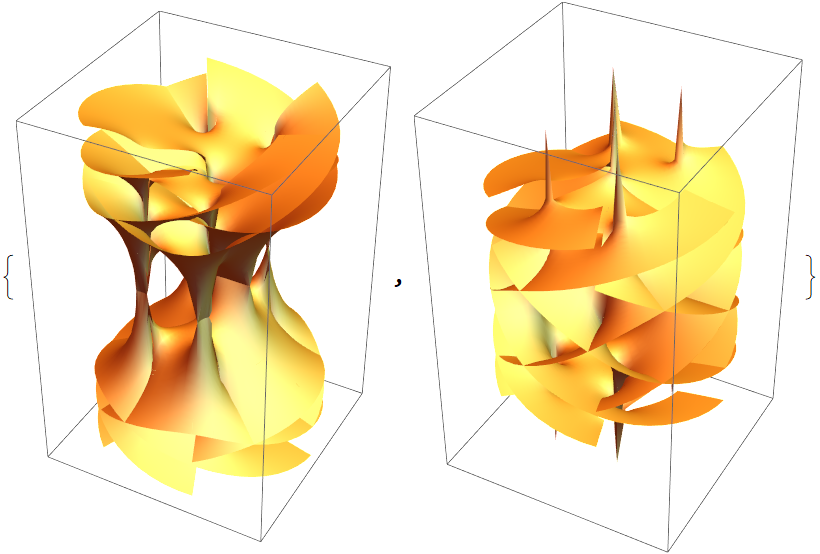
![{ ResourceFunction["RiemannSurfacePlot3D"][w == Sqrt[Sqrt[z] + z^2], Im[w], {z, w}, ViewPoint -> {-3.08, -1.035, 0.940}],
ResourceFunction["RiemannSurfacePlot3D"][
w == Sqrt[z - Sqrt[z^3 - 1]], Re[w], {z, w}, ViewPoint -> {-2.98, 1.33, 0.89}]}](https://www.wolframcloud.com/obj/resourcesystem/images/540/5409a3e7-a791-40b6-9f12-75d6be8fa109/7731b792c912fe77.png)


![ContourPlot3D[
Evaluate[xyvResultant == 0], {x, -1.2, 1.2}, {y, -1.2, 1.2}, {v, -1.4, 1.4}, PlotPoints -> 60,
RegionFunction -> (Norm[{#1, #2}] <= 1.2 &), Mesh -> None, BoxRatios -> {1, 1, 1.61}, Axes -> False, PlotRange -> All]](https://www.wolframcloud.com/obj/resourcesystem/images/540/5409a3e7-a791-40b6-9f12-75d6be8fa109/2b6275f437904649.png)
![Show[Table[
Plot3D[Evaluate[ Im[Exp[2 Pi I j/4] (1 - (x + I y)^4)^(1/4)]] , {x, -1.2, 1.2}, {y, -1.2, 1.2},
RegionFunction -> (Norm[{#1, #2}] <= 1.2 &),
PlotRange -> All, Mesh -> None, BoxRatios -> {1, 1, 1.61}, Axes -> False],
{j, 0, 3}]]](https://www.wolframcloud.com/obj/resourcesystem/images/540/5409a3e7-a791-40b6-9f12-75d6be8fa109/5666a58c080897d9.png)
![ResourceFunction["RiemannSurfacePlot3D"][
w == Sqrt[ArcCos[z]/ArcSin[z]], Re[w], {z, w}, ViewPoint -> {3, -3, 0}]](https://www.wolframcloud.com/obj/resourcesystem/images/540/5409a3e7-a791-40b6-9f12-75d6be8fa109/1df03d072955afb2.png)
![plasterModelImage = ImageTake[
Import["http://modellsammlung.uni-goettingen.de/data/Large/i252_2.jpg"], {30, -5}, {250, 1200}];](https://www.wolframcloud.com/obj/resourcesystem/images/540/5409a3e7-a791-40b6-9f12-75d6be8fa109/2faf6445e54f6850.png)
![GraphicsRow[{Show[plasterModelImage, ImageSize -> 320], ResourceFunction["RiemannSurfacePlot3D"][w == Sqrt[z^2 - 1], Im[w], {z, w},
BoxRatios -> {1, 1, 1}, PlotStyle -> GrayLevel[0.7], ViewPoint -> {2.85, 0.75, 1.6},
Lighting -> "Neutral", Boxed -> False, Background -> GrayLevel[0.25]]}]](https://www.wolframcloud.com/obj/resourcesystem/images/540/5409a3e7-a791-40b6-9f12-75d6be8fa109/7c6aea34ec05730c.png)
![{ResourceFunction["RiemannSurfacePlot3D"][
w == Sqrt[1 - z^4]/Log[1 - z^6], Re[w], {z, w}, PlotStyle -> Opacity[0.8]],
ResourceFunction["RiemannSurfacePlot3D"][
w == Log[1 - z^4]/Sqrt[1 - z^6], Re[w], {z, w}, PlotStyle -> Opacity[0.8]]}](https://www.wolframcloud.com/obj/resourcesystem/images/540/5409a3e7-a791-40b6-9f12-75d6be8fa109/125fe7a584eb78af.png)
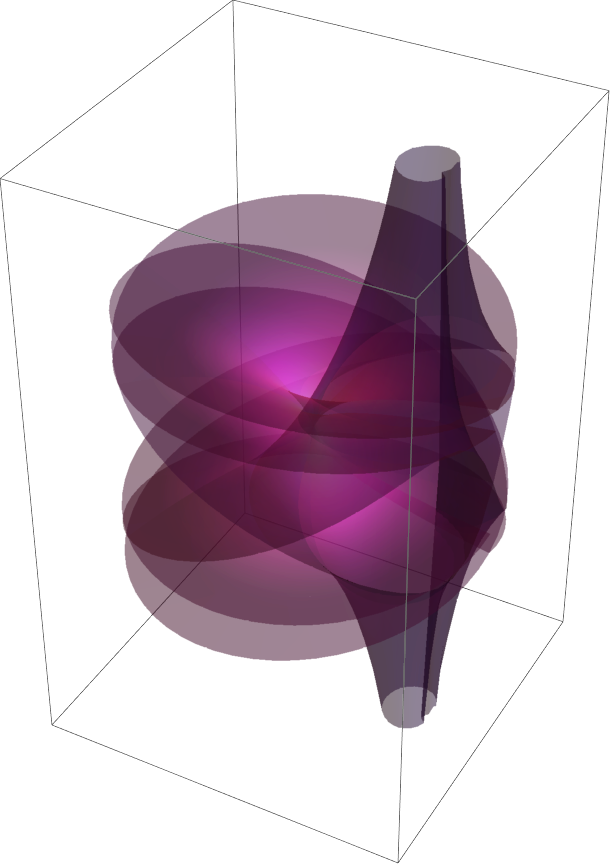
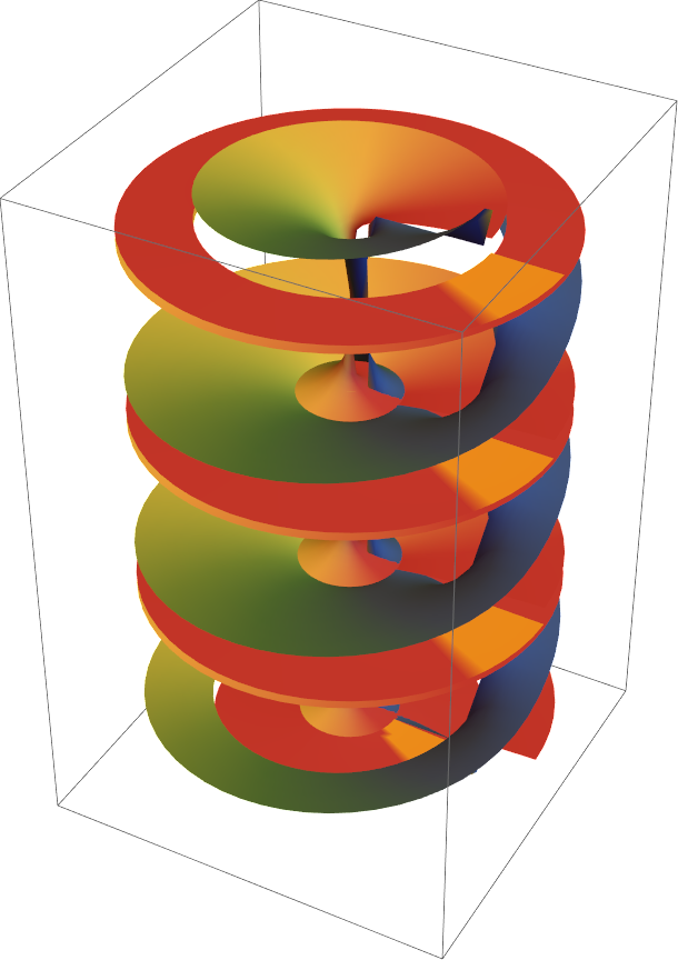
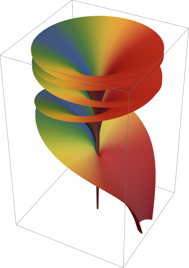
![ResourceFunction["RiemannSurfacePlot3D"][
w == Sqrt[Log[z]], {Re[z], Im[w], Im[z]}, {z, w},
LogSheets -> Range[-3, 3], ViewPoint -> {1.4, 0, -3.08}, BoxRatios -> {1, 3, 1},
PlotStyle -> Directive[GrayLevel[0.4], Specularity[Red, 12]]]](https://www.wolframcloud.com/obj/resourcesystem/images/540/5409a3e7-a791-40b6-9f12-75d6be8fa109/6f4e6b997c859fea.png)

![ResourceFunction["RiemannSurfacePlot3D"][w == Power[I - z^4, (4)^-1], Im[w], {z, w}, ColorFunction -> (Directive[Opacity[0.6], Hue[(Arg[#2] + Pi)/(2 Pi)]] &),
PlotPoints -> {90, 60}, Boxed -> False]](https://www.wolframcloud.com/obj/resourcesystem/images/540/5409a3e7-a791-40b6-9f12-75d6be8fa109/6dbbf69148fce0f7.png)
![ResourceFunction["RiemannSurfacePlot3D"][
w == Log[ Sqrt[z] + Power[z, (3)^-1] ], Re[w], {z, w}, "LogSheets" -> Range[-3, 3], ColorFunction -> (ColorData["DarkRainbow"][Cos[Arg[#1]/2]] &)]](https://www.wolframcloud.com/obj/resourcesystem/images/540/5409a3e7-a791-40b6-9f12-75d6be8fa109/56dceffbd1728dd8.png)
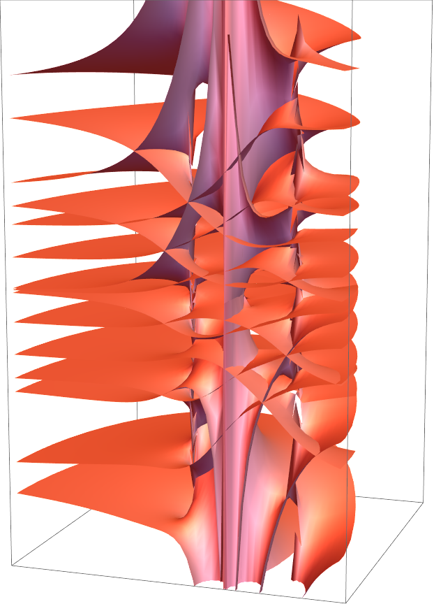
![Show[ResourceFunction["RiemannSurfacePlot3D"][
w == (ArcTan[z] + ArcTan[\[Pi] - z])/ArcTan[\[Pi]/2 - z], Re[w], {z, w}, "LogSheets" -> {-1, 0},
PlotStyle -> Directive[ Pink, Specularity[Pink, 6]]], PlotRange -> {All, {0, 6}, {-6, 6}}, ViewPoint -> {1, -3, 0.5}]](https://www.wolframcloud.com/obj/resourcesystem/images/540/5409a3e7-a791-40b6-9f12-75d6be8fa109/1df67567e30e7f3b.png)
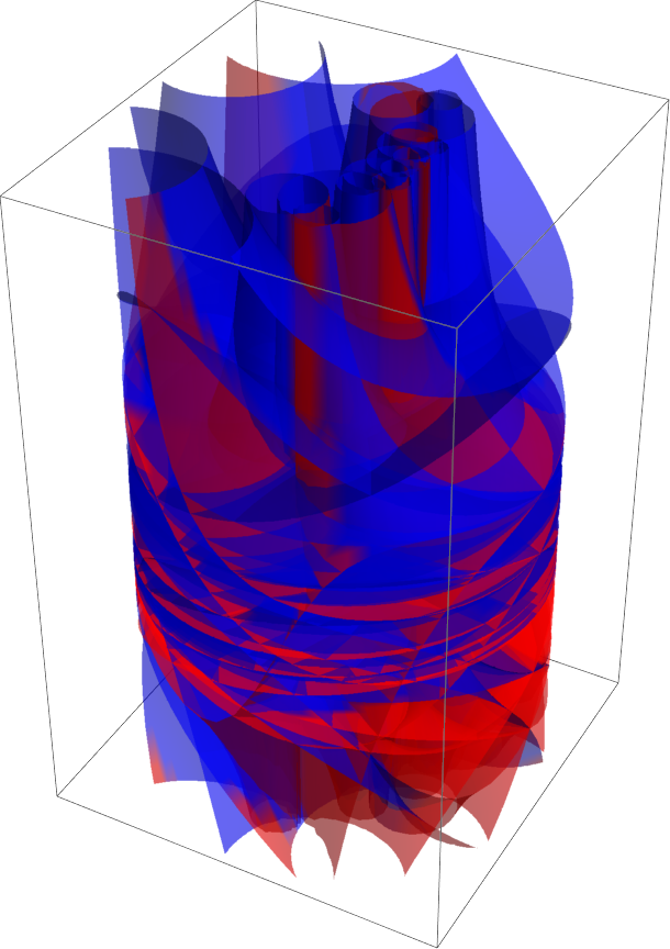
![ResourceFunction["RiemannSurfacePlot3D"][
w == (1 + Power[z, (3)^-1])/(1 + Sqrt[z] + Power[z^5, (6)^-1]), Re[w], {z, w}, ColorFunction -> (Directive[Opacity[0.6], If[Re[#2] > Im[#2], Blue, Red]] &)]](https://www.wolframcloud.com/obj/resourcesystem/images/540/5409a3e7-a791-40b6-9f12-75d6be8fa109/7e4eccfc395f73e5.png)
![{ResourceFunction["RiemannSurfacePlot3D"][
w == Sqrt[Log[z + z^3 + z^5]], Re[w], {z, w}],
ResourceFunction["RiemannSurfacePlot3D"][
w == Sqrt[Log[z + z^3 + z^5]], Im[w], {z, w}]}](https://www.wolframcloud.com/obj/resourcesystem/images/540/5409a3e7-a791-40b6-9f12-75d6be8fa109/5c80b3de8801cc4e.png)
![ResourceFunction["RiemannSurfacePlot3D"][
w == (Sqrt[z + 1] - Sqrt[z - 1])/(Sqrt[z + I] + Sqrt[z - I]), Re[w], {z, w}, ColorFunction -> (ColorData["GreenBrownTerrain"][RandomReal[]] &), ViewPoint -> {3.03, -1.51, 0.12}]](https://www.wolframcloud.com/obj/resourcesystem/images/540/5409a3e7-a791-40b6-9f12-75d6be8fa109/513abf1d674ad0b8.png)
![rs = ResourceFunction["RiemannSurfacePlot3D"][
w == Power[z, (3)^-1]/(6 + Sqrt[z - 1]) , Im[w], {z, w}, PlotPoints -> {80, 40}, ColorFunction -> (Directive[Opacity[0.8], ColorData["AuroraColors"][Cos[ Arg[2 #2] /2]]] &)]](https://www.wolframcloud.com/obj/resourcesystem/images/540/5409a3e7-a791-40b6-9f12-75d6be8fa109/0271f166fa5a65bc.png)
![roughen[expr_, scale_] := Module[{gcs = Cases[expr, _GraphicsComplex, {0, Infinity}], \[CurlyEpsilon] = 0.001, pts, ptsGroups, newP, L},
pts = Union[Flatten[First /@ gcs, 1]];
L = Max[Abs[Subtract @@@ MinMax /@ Transpose[pts]]];
ptsGroups = {#[[1, 1]], Last /@ #} & /@ Split[Sort[{Round[#, \[CurlyEpsilon]], #} & /@ pts], #1[[1]] === #2[[1]] &];
Function[{p, ps}, With[{\[DoubleStruckR] = scale L RandomVariate[NormalDistribution[]] Normalize[
RandomReal[{-1, 1}, 3]]}, (newP[#] = p + \[DoubleStruckR]) & /@ ps]] @@@ ptsGroups;
expr /. GraphicsComplex[l_, rest__] :> GraphicsComplex[newP /@ l, Sequence @@ DeleteCases[{rest}, VertexNormals -> _, {0, Infinity}]]]](https://www.wolframcloud.com/obj/resourcesystem/images/540/5409a3e7-a791-40b6-9f12-75d6be8fa109/600f0859e72c0ea0.png)
![ResourceFunction["RiemannSurfacePlot3D"][w == Power[1 + z^4, (4)^-1],
Re[w], {z, w}, BoxRatios -> {1, 1, 1}, PlotStyle -> Opacity[0.8], Boxed -> False] /. GraphicsComplex[pts_, __] :> ListPlot3D[pts, PlotStyle -> Texture[Entity["Country", "UnitedKingdom"][
EntityProperty["Country", "Flag"]]],
Mesh -> None, BoundaryStyle -> None, PlotRange -> All][[1]]](https://www.wolframcloud.com/obj/resourcesystem/images/540/5409a3e7-a791-40b6-9f12-75d6be8fa109/5908986876702aa5.png)
![ResourceFunction["RiemannSurfacePlot3D"][
w == Log[(7 - 2 z + z^3)/Sqrt[-1 + z - 3 z^3 + z^5]], Im[w], {z, w}, ViewPoint -> {1.12, -3.03, 1.02}, "ShowBranchPoints" -> True,
ColorFunction -> (Directive[Orange, Opacity[Piecewise[{{1, Im[#2] < -8}, {1 - ((Im[#2] + 8)/18)^0.25,
Im[#2] > -8}}]]] &)]](https://www.wolframcloud.com/obj/resourcesystem/images/540/5409a3e7-a791-40b6-9f12-75d6be8fa109/306ad1a6c4fc9812.png)

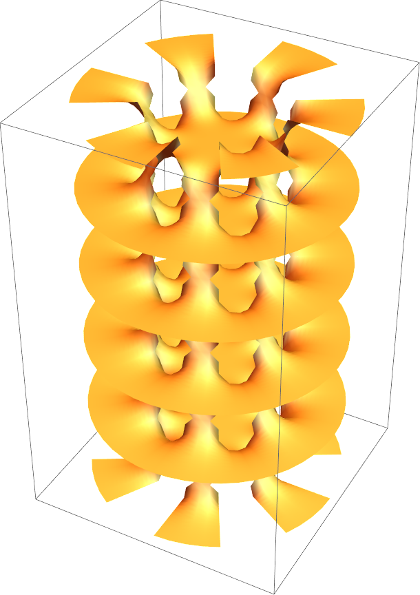
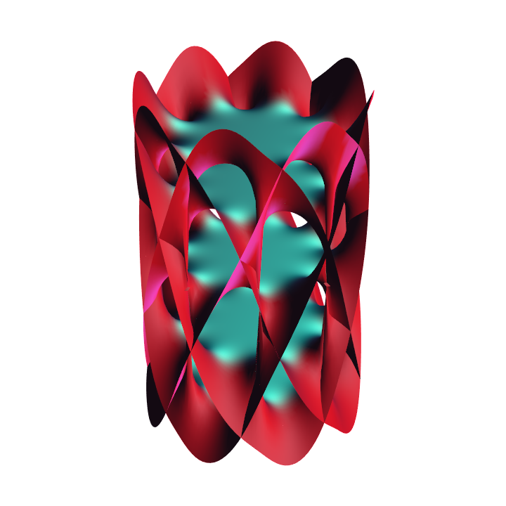
![ResourceFunction["RiemannSurfacePlot3D"][w == Power[1 - z^8, (5)^-1], Im[w], {z, w}, "BranchPointPlotRangeFactor" -> 1.2,
PlotPoints -> {180, 32}, Boxed -> False, SphericalRegion -> True, ViewPoint -> Dynamic[{3 Cos[Clock[2 Pi]], 3 Sin[Clock[2 Pi]], 1 + Abs[ Sin[Clock[Pi]]]}, UpdateInterval -> 0], PlotStyle -> Directive[RGBColor[
0.8873402883377823, 0.0881874778872287, 0.20269962280609732`], Specularity[RGBColor[
0.00826013975092077, 0.9983549796506077, 0.8536693247046465], 12]], Lighting -> {{"Ambient", RGBColor[
0.08991790342148565, 0.4656695106684785, 0.3563096997888613]}, {"Directional", RGBColor[
0.58565433989252, 0.20711472123320362`, 0.6773803713053297], ImageScaled[{1, -1, -2}]}, {"Directional", RGBColor[
0.9340004634836698, 0.21091405108492345`, 0.24376150618256442`], ImageScaled[{3, -1, 3}]}, {"Directional", RGBColor[
0.01234965817203082, 0.8702599913137037, 0.7827905082641344], ImageScaled[{1, 3, -1}]}}]](https://www.wolframcloud.com/obj/resourcesystem/images/540/5409a3e7-a791-40b6-9f12-75d6be8fa109/282e64ff662decc4.png)
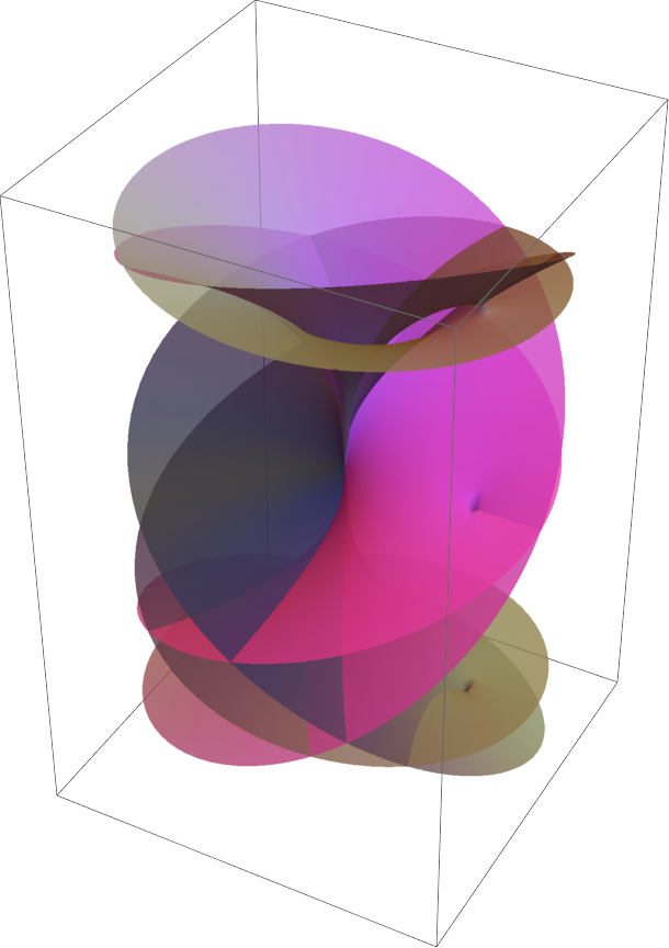
![With[{colors = Table[RandomColor[], {100}]},
Manipulate[
ResourceFunction["RiemannSurfacePlot3D"][
z + w + z w + z^2 + 1/w + 1/z == 1, Re[w], {z, w},
PlotStyle -> colors, ClipPlanes -> InfinitePlane[{0, y, 0}, {{0, 0, 1}, {1, 0, 0}}]],
{{y, 0, "cut plane"}, -3, 3}]]](https://www.wolframcloud.com/obj/resourcesystem/images/540/5409a3e7-a791-40b6-9f12-75d6be8fa109/40ebd18f80803838.png)
![Manipulate[
ResourceFunction["RiemannSurfacePlot3D"][
w == Sqrt[1 - z^3], (1 - \[Sigma]) Re[w] + \[Sigma] Im[w], {z, w},
PlotStyle -> Directive[Opacity[0.8], Blue, Specularity[Yellow, 12]]],
Row[{"Re", Control[{{\[Sigma], 0, ""}, 0, 1}], " Im"}]]](https://www.wolframcloud.com/obj/resourcesystem/images/540/5409a3e7-a791-40b6-9f12-75d6be8fa109/511f297dbe7fdb64.png)
![Manipulate[
ResourceFunction["RiemannSurfacePlot3D"][
w == (Sqrt[z - 1] Sqrt[z + 1])/(
Sqrt[z - 1] - Sqrt[
z + 1]), {\[CurlyPhi]xy, \[CurlyPhi]xu, \[CurlyPhi]xv, \[CurlyPhi]yu, \[CurlyPhi]yv, \[CurlyPhi]uv}, {z, w}], Row[{"show ", Button["u(x,y)", {\[CurlyPhi]xy, \[CurlyPhi]xu, \[CurlyPhi]xv, \[CurlyPhi]yu, \[CurlyPhi]yv, \[CurlyPhi]uv} = {0, 0, 0, 0, 0, 0}], Button["v(x,y)", {\[CurlyPhi]xy, \[CurlyPhi]xu, \[CurlyPhi]xv, \[CurlyPhi]yu, \[CurlyPhi]yv, \[CurlyPhi]uv} = {0, 0, 0, 0, 0, \[Pi]/2}]}],
Row[{"show ", Button["x(u,v)", {\[CurlyPhi]xy, \[CurlyPhi]xu, \[CurlyPhi]xv, \[CurlyPhi]yu, \[CurlyPhi]yv, \[CurlyPhi]uv} = {0, \[Pi]/2, \[Pi], 0, \[Pi]/2, 0}],
Button[
"y(u,v)", {\[CurlyPhi]xy, \[CurlyPhi]xu, \[CurlyPhi]xv, \[CurlyPhi]yu, \[CurlyPhi]yv, \[CurlyPhi]uv} = {0, 0, \[Pi]/2, \[Pi]/2, \[Pi], \[Pi]/2}] }],
{{\[CurlyPhi]xy, 0, "\!\(\*SubscriptBox[\(\[CurlyPhi]\), \(x, y\)]\)"}, -Pi, Pi}, {{\[CurlyPhi]xu, 0, "\!\(\*SubscriptBox[\(\[CurlyPhi]\), \(x, u\)]\)"}, -Pi, Pi},
{{\[CurlyPhi]xv, 0, "\!\(\*SubscriptBox[\(\[CurlyPhi]\), \(x, v\)]\)"}, -Pi, Pi}, {{\[CurlyPhi]yu, 0, "\!\(\*SubscriptBox[\(\[CurlyPhi]\), \(y, u\)]\)"}, -Pi, Pi},
{{\[CurlyPhi]yv, 0, "\!\(\*SubscriptBox[\(\[CurlyPhi]\), \(y, v\)]\)"}, -Pi, Pi}, {{\[CurlyPhi]uv, 0, "\!\(\*SubscriptBox[\(\[CurlyPhi]\), \(u, v\)]\)"}, -Pi, Pi},
ControlPlacement -> Left]](https://www.wolframcloud.com/obj/resourcesystem/images/540/5409a3e7-a791-40b6-9f12-75d6be8fa109/1ac50cd275efd54c.png)