Wolfram Function Repository
Instant-use add-on functions for the Wolfram Language
Function Repository Resource:
Visualize a complex function as an array of bubbles
ResourceFunction["ComplexBubblePlot"][f,{z,zmin,zmax}] generates a plot of f as an array of disks scaled by Abs[f], over the complex rectangle with corners zmin and zmax. |
| ColorFunction | Automatic | how to apply coloring to disks |
| ColorFunctionScaling | True | whether to scale arguments to ColorFunction |
| Frame | Automatic | whether to put a frame around the plot |
| PlotLegends | None | legends for color gradients |
| PlotPoints | Automatic | the number of disks in each direction |
| PlotRange | Automatic | range of values to include |
| PlotRangeClipping | True | whether to clip at the plot range |
| WorkingPrecision | MachinePrecision | the precision used in internal computations |
Plot a complex function:
| In[1]:= |
| Out[1]= | 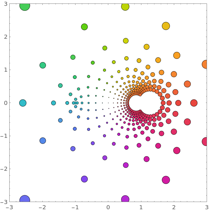 |
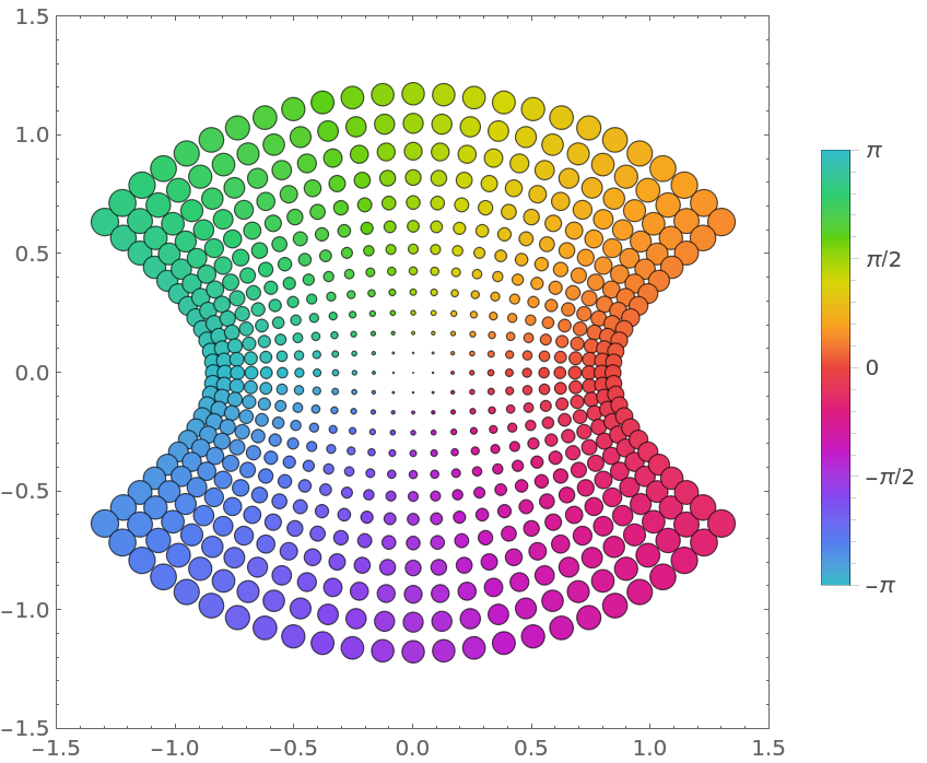
Include a legend showing how the colors vary from -π to π:
| In[2]:= |
| Out[2]= | 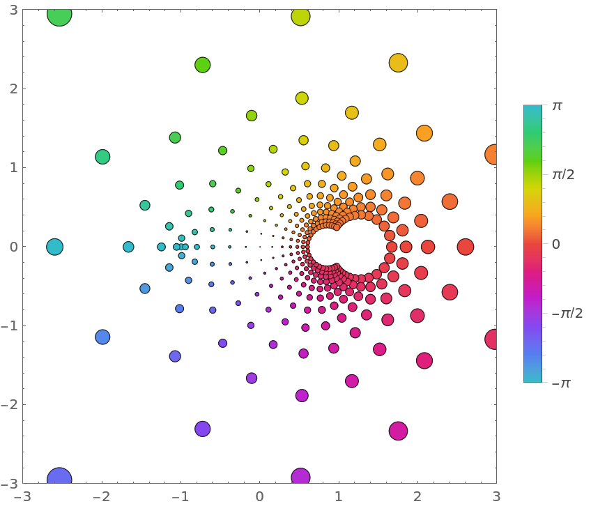 |
The identity function:
| In[3]:= |
| Out[3]= | 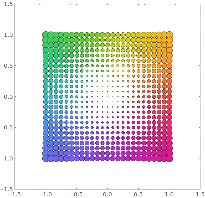 |
Visualize various Power functions:
| In[4]:= | ![Table[ResourceFunction["ComplexBubblePlot"][z^a, {z, -1 - I, 1 + I}, PlotLabel -> ToString[z^a, TraditionalForm]], {a, {-1, 1/2, 2, 3}}] // Partition[#, 2] & // GraphicsGrid](https://www.wolframcloud.com/obj/resourcesystem/images/639/6396746d-50b4-4a47-bb6e-d1904d0d46bf/223e867ee7fa2f7e.png) |
| Out[4]= | 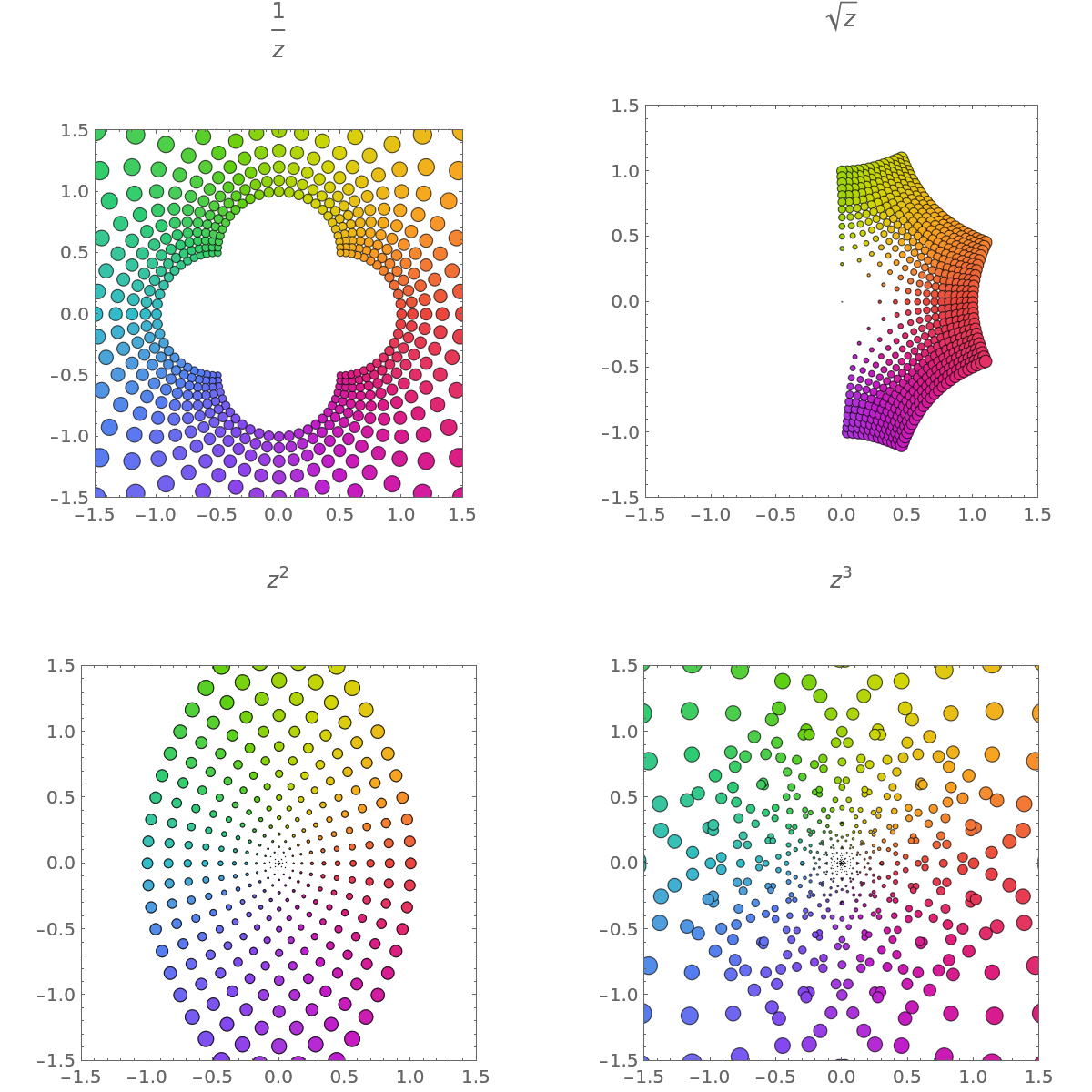 |
Visualize a function with an essential singularity:
| In[5]:= |
| Out[5]= | 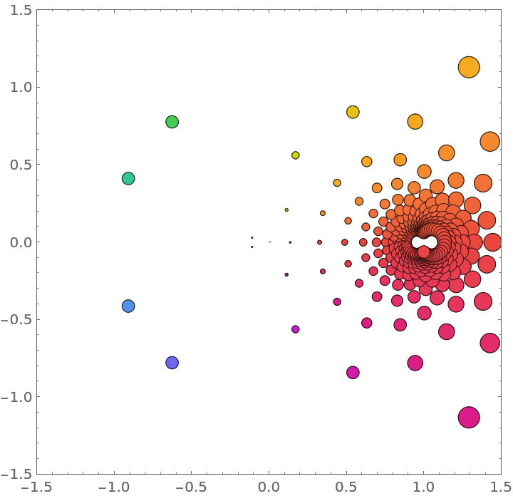 |
Use a different color function:
| In[6]:= |
| Out[6]= | 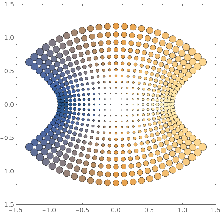 |
Arg[f] is scaled by default. Use ColorFunctionScaling to change it:
| In[7]:= |
| Out[7]= | 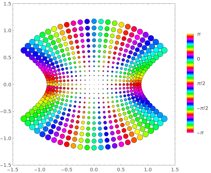 |
Use more disks:
| In[9]:= |
| Out[9]= | 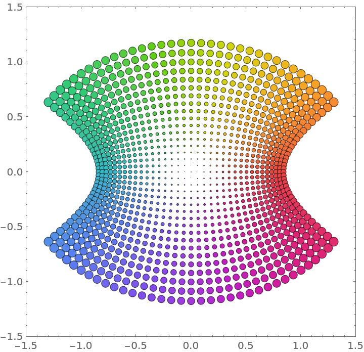 |
Evaluate functions using arbitrary-precision arithmetic:
| In[10]:= |
| Out[10]= | 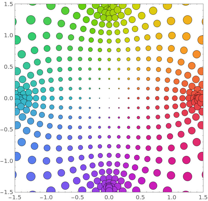 |
Visualize the function -ⅈza with varying a:
| In[11]:= | ![Manipulate[
ResourceFunction["ComplexBubblePlot"][-I z^a, {z, 1}, ColorFunction -> (ColorData["M10DefaultDensityGradient", 1 - Abs[2 Mod[#, 1] - 1]] &)], {{a, 1}, 0.1, 4, 0.1}, SaveDefinitions -> True]](https://www.wolframcloud.com/obj/resourcesystem/images/639/6396746d-50b4-4a47-bb6e-d1904d0d46bf/4f54f7ab51ca2db0.png) |
| Out[11]= | 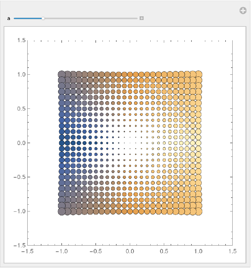 |
This work is licensed under a Creative Commons Attribution 4.0 International License