Wolfram Function Repository
Instant-use add-on functions for the Wolfram Language
Warning: This resource is provisional
Function Repository Resource:
Dynamically visualize an ordinary differential equation (ODE) or system of ODEs
ResourceFunction["ODEViewer"][eqns, init, deps, {t}] creates a dynamic visualization and computes properties of the ordinary differential equation system eqns, with initial conditions init, written in terms of dependent variables deps and independent variable t. | |
ResourceFunction["ODEViewer"][eqns, init, dep, {t, t1, t2}] creates a dynamic visualization of eqns with t varying from t1 to t2. |
Visualize the slope field of a simple equation and it's solution for a given initial condition:
| In[1]:= |
| Out[1]= | 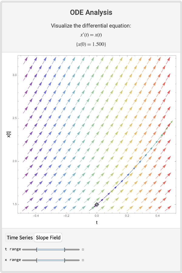 |
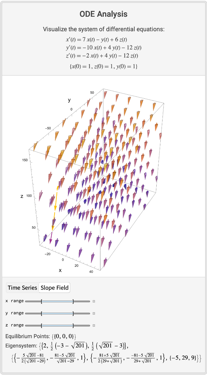
Visualize a system in three dimensions:
| In[2]:= | ![ResourceFunction["ODEViewer", ResourceVersion->"1.0.0"][{Derivative[1][x][t] == 7 x[t] - y[t] + 6 z[t], Derivative[1][y][t] == -10 x[t] + 4 y[t] - 12 z[t], Derivative[1][z][t] == -2 x[t] + 4 y[t] - 12 z[t]}, {x[0] == 1, z[0] == 1, y[0] == 1}, {x, y, z}, {t, 0, 5}]](https://www.wolframcloud.com/obj/resourcesystem/images/21d/21db79b7-a20d-4613-9c90-ffd6b5c39d24/1-0-0/52e3df7f831f16de.png) |
Visualize the slope field for a non-linear system:
| In[3]:= |
| Out[3]= | 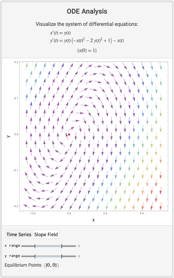 |
A stiff system:
| In[4]:= | ![ResourceFunction["ODEViewer", ResourceVersion->"1.0.0"][{Derivative[1][x][t] == y[t], Derivative[1][y][t] == -x[t] - 2 y[t] - y[t]^3}, {x[0] == 0, y[0] == 1, WhenEvent[y[t] > 10, "StopIntegration"]}, {x, y}, {t, 0, 1}]](https://www.wolframcloud.com/obj/resourcesystem/images/21d/21db79b7-a20d-4613-9c90-ffd6b5c39d24/1-0-0/7068b99ae5fb677b.png) |
| Out[4]= | 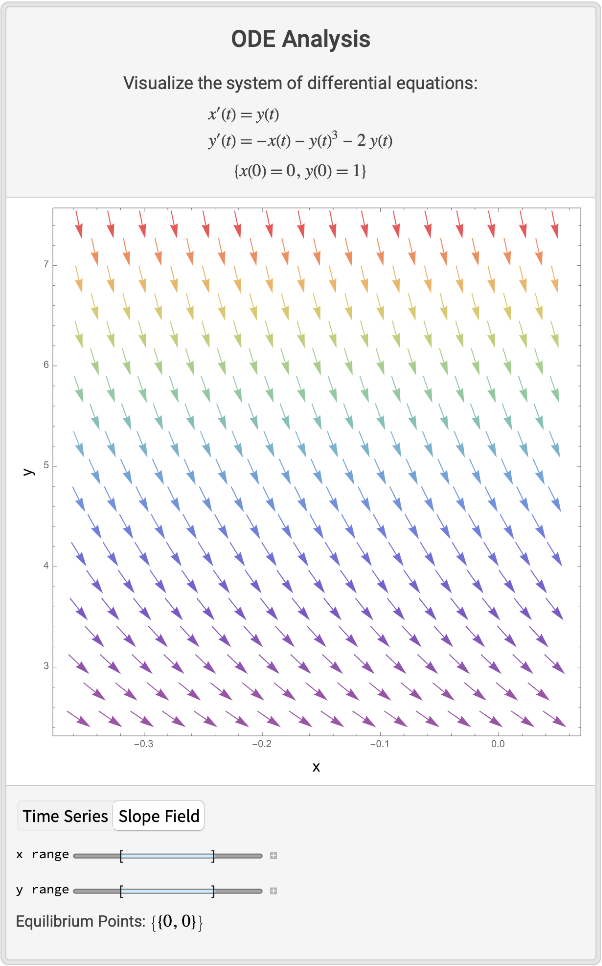 |
A multiple solution case:
| In[5]:= |
| Out[5]= | 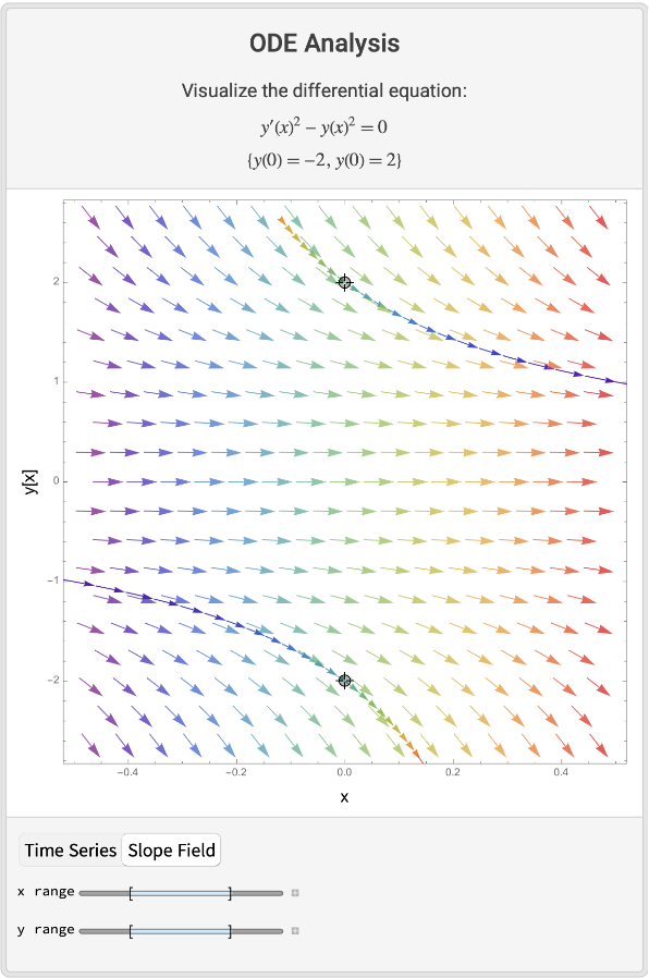 |
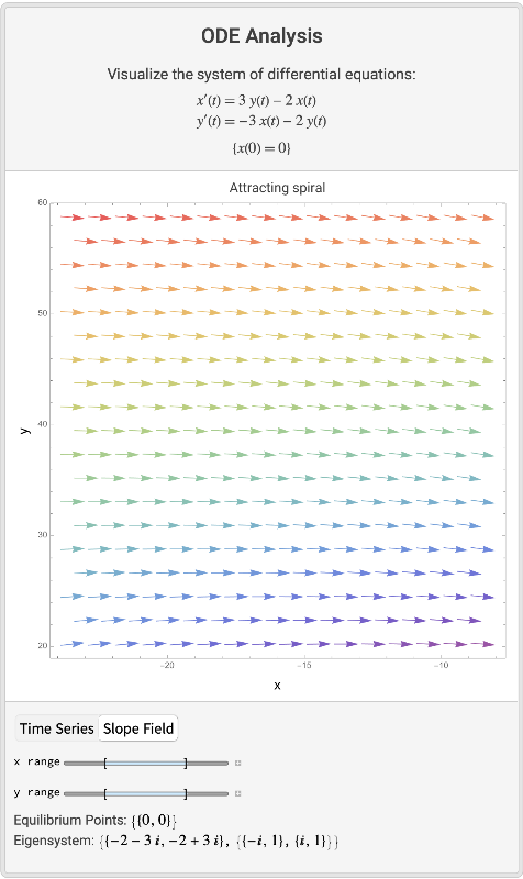
A linear system, the plot range is calculated automatically, but the plot range is not optimal:
| In[6]:= |
The same system, with a explicit plot range:
| In[7]:= |
| Out[7]= | 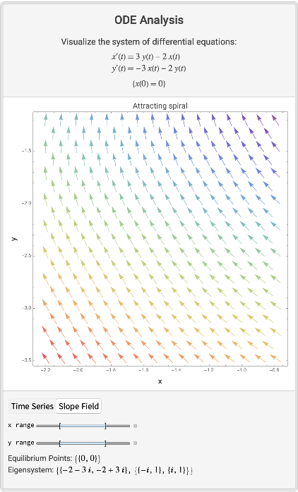 |
If something fails shows nothing:
| In[8]:= | ![ResourceFunction["ODEViewer", ResourceVersion->"1.0.0"][{Derivative[1][y][x] == (2 (1/x - 1/x^2))/(
y[x] - 1/y[x])}, {y[1] == -1}, {y}, {x, .1, 1}]](https://www.wolframcloud.com/obj/resourcesystem/images/21d/21db79b7-a20d-4613-9c90-ffd6b5c39d24/1-0-0/283e04bed7bd066d.png) |
| Out[8]= | 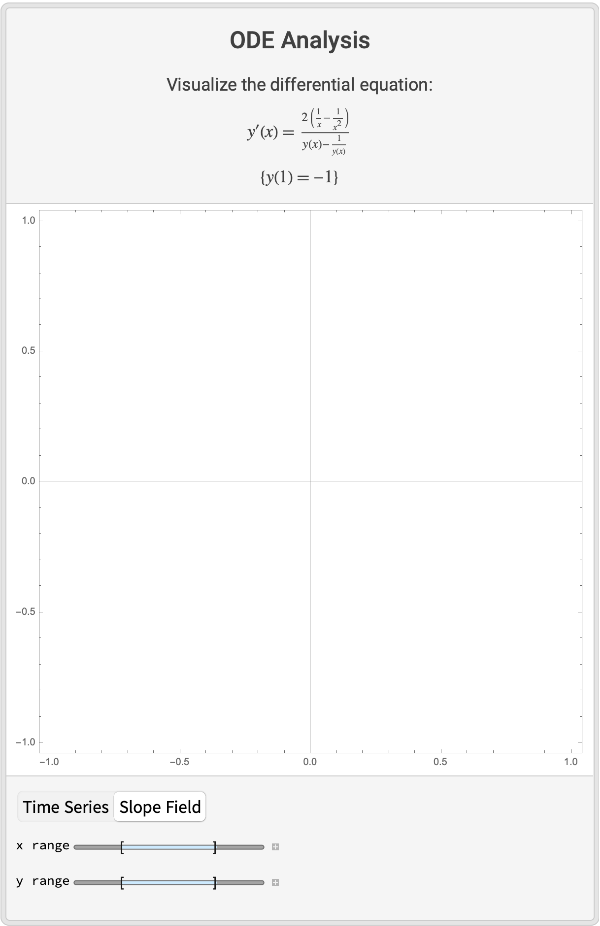 |
To view the full source code for ODEViewer, evaluate the following:
This work is licensed under a Creative Commons Attribution 4.0 International License