Function Repository Resource:

CubicMonotonicInterpolation

Source Notebook

Interpolate data with a monotonic piecewise cubic Hermite interpolant

Contributed by: Jan Mangaldan

ResourceFunction["CubicMonotonicInterpolation"][{f1,f2,}]

constructs a monotonic cubic Hermite interpolation of the function values fi, assumed to correspond to x values 1, 2, ….

ResourceFunction["CubicMonotonicInterpolation"][{{x1,f1},{x2,f2},}]

constructs a monotonic cubic Hermite interpolation of the function values fi corresponding to x values xi.

Details and Options

ResourceFunction["CubicMonotonicInterpolation"] returns an InterpolatingFunction object, which can be used like any other pure function.
The interpolation function returned by ResourceFunction["CubicMonotonicInterpolation"][data] is set up so as to agree with data at every point explicitly specified in data.
If data is monotonic, ResourceFunction["CubicMonotonicInterpolation"] yields an interpolant that preserves the monotonicity of the data.
The function values fi are expected to be real or complex numbers.
The function arguments xi must be real numbers.
ResourceFunction["CubicMonotonicInterpolation"][data] generates an InterpolatingFunction object that returns values with the same precision as those in data.
ResourceFunction["CubicMonotonicInterpolation"] takes the following options:
MethodAutomaticmethod to use
PeriodicInterpolationFalsewhether to treat the data as periodic
Possible settings for Method include "Steffen", "FritschCarlson" and "Stineman", with the default being Automatic.
With the setting PeriodicInterpolationTrue, only the data for a single fundamental period are required.

Examples

Basic Examples (3) 

Construct an approximate function that interpolates the data:

In[1]:=
f = ResourceFunction[
  "CubicMonotonicInterpolation"][{0., 0.6, 1., 1.3, 1.4, 2.1}]
Out[1]=

Apply the function to find interpolated values:

In[2]:=
f[3.7]
Out[2]=

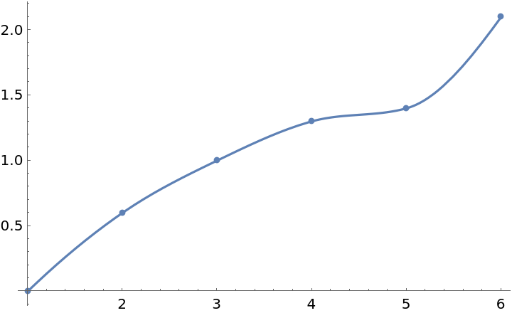
Plot the interpolation function along with the original data:

In[3]:=
Show[Plot[f[x], {x, 1, 6}], ListPlot[{0., 0.6, 1., 1.3, 1.4, 2.1}]]
Out[3]=

Scope (2) 

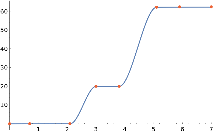
Interpolate and plot a monotonic data set:

In[4]:=
data = {{0., 0.}, {0.7, 0.02}, {2.1, 0.06}, {3., 20.}, {3.8, 20.}, {5.1, 62.2}, {5.9, 62.24}, {7., 62.26}};
fun = ResourceFunction["CubicMonotonicInterpolation"][data]
Out[4]=
In[5]:=
Plot[fun[x], {x, 0, 7}, Epilog -> {Directive[AbsolutePointSize[5], ColorData[97, 4]], Point[data]}]
Out[5]=

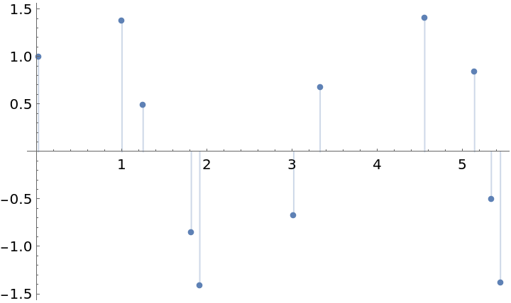
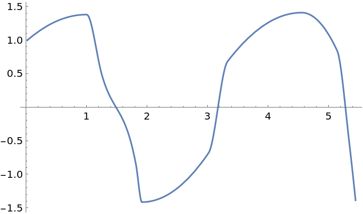
Form an interpolation from data given as a TimeSeries:

In[6]:=
ts = TemporalData[
  TimeSeries, {{{1, Cos[1] + Sin[1], Cos[2] + Sin[2], Cos[3] + Sin[3],
       Cos[4] + Sin[4], Cos[5] + Sin[5], Cos[6] + Sin[6], Cos[7] + Sin[7], Cos[8] + Sin[8], Cos[9] + Sin[9], Cos[10] + Sin[10]}}, {{{0.016965744360214943`, 0.9973865299845299, 1.24591736467102, 1.8114088692820352`, 1.9107450982712126`, 3.013995043949912, 3.323754146542503, 4.551557869716615, 5.13709169763333, 5.334143602077121, 5.441221219515277}}}, 1, {"Continuous", 1}, {"Discrete", 1}, 1, {ResamplingMethod -> {"Interpolation", InterpolationOrder -> 1}}},
    False, 10.1];
In[7]:=
ListPlot[ts, Filling -> Axis]
Out[7]=
In[8]:=
fun = ResourceFunction["CubicMonotonicInterpolation"][ts]
Out[8]=
In[9]:=
Plot[fun[x], {x, ts["FirstTime"], ts["LastTime"]}]
Out[9]=

Options (2) 

Method (1) 

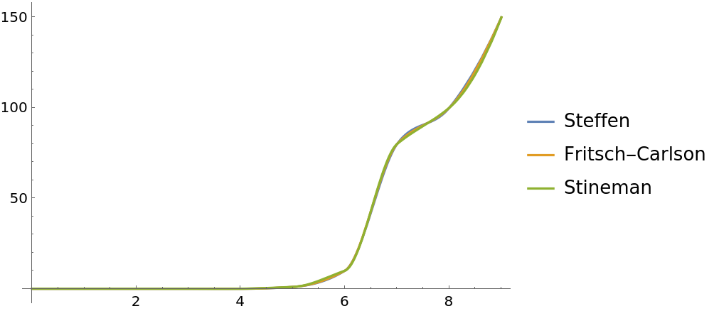
Compare different monotonic interpolation methods:

In[10]:=
data = {{0., 0.}, {1., 0.}, {2., 0.}, {3., 0.}, {4., 0.}, {5., 1.}, {6., 10.}, {7., 80.}, {8., 100.}, {9., 150.}};
In[11]:=
fSte = ResourceFunction["CubicMonotonicInterpolation"][data, Method -> "Steffen"];
fFC = ResourceFunction["CubicMonotonicInterpolation"][data, Method -> "FritschCarlson"];
fSti = ResourceFunction["CubicMonotonicInterpolation"][data, Method -> "Stineman"];
In[12]:=
Plot[{fSte[x], fFC[x], fSti[x]}, {x, 0, 9}, PlotLegends -> {"Steffen", "Fritsch-Carlson", "Stineman"}]
Out[12]=

PeriodicInterpolation (1) 

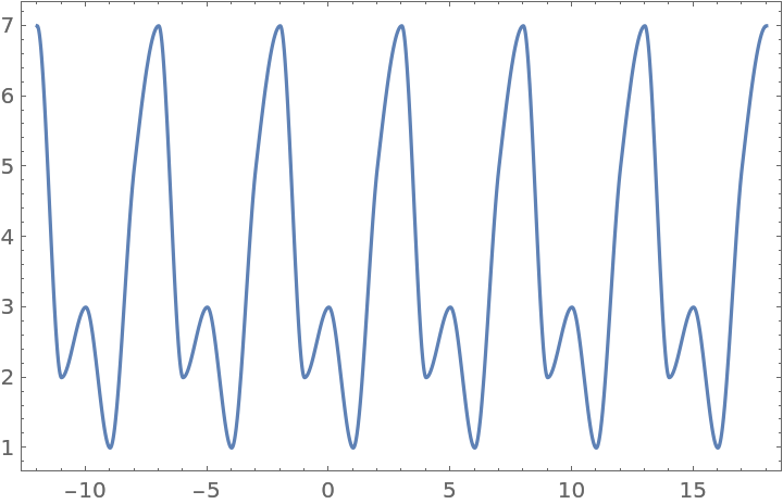
With PeriodicInterpolation->True, the data is interpreted as one period of a periodic function:

In[13]:=
fp = ResourceFunction[
  "CubicMonotonicInterpolation"][{1, 5, 7, 2, 3, 1}, PeriodicInterpolation -> True]
Out[13]=
In[14]:=
Plot[fp[x], {x, -12, 18}, {Axes -> None, Frame -> True}]
Out[14]=

Properties and Relations (2) 

A monotonic data set:

In[15]:=
data = {{0., 0.}, {0.0057269, 0.2}, {0.0366617, 0.4}, {0.158682, 0.6}, {0.50688, 0.8}, {1., 1.}};
In[16]:=
fHerm = Interpolation[data, Method -> "Hermite"];
fSpl = Interpolation[data, Method -> "Spline"];
fMon = ResourceFunction["CubicMonotonicInterpolation"][data];

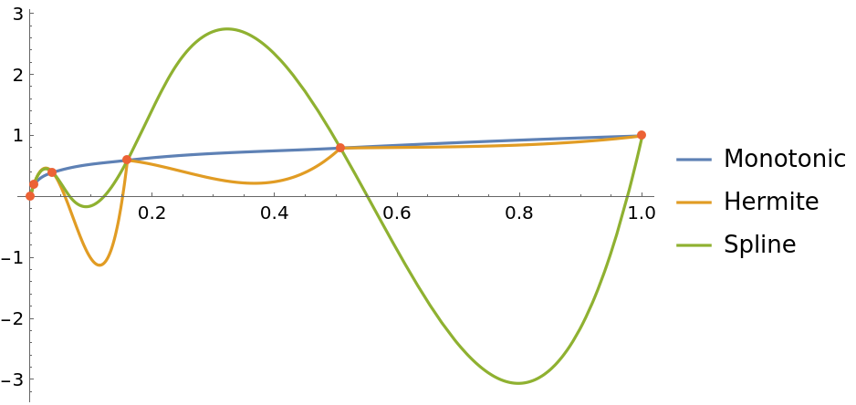
Compare CubicMonotonicInterpolation with the built-in "Hermite" and "Spline" methods of Interpolation. The built-in methods do not preserve monotonicity, and give spurious oscillations:

In[17]:=
Plot[{fMon[x], fHerm[x], fSpl[x]}, {x, 0, 1}, Epilog -> {Directive[AbsolutePointSize[5], ColorData[97, 4]], Point[data]}, PlotLegends -> {"Monotonic", "Hermite", "Spline"}, PlotRange -> All]
Out[17]=

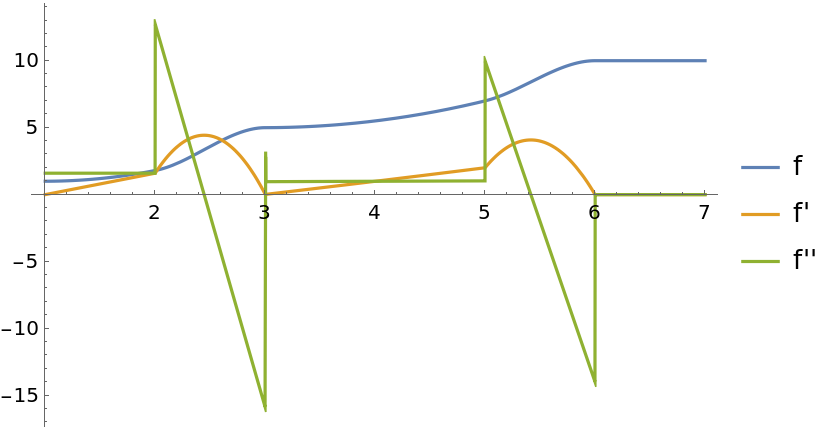
The interpolant returned by CubicMonotonicInterpolation is continuous up to its first derivative:

In[18]:=
data = {{1., 1.}, {2., 1.8}, {3., 5.}, {3.006, 5.0001}, {5., 7.}, {6.,
     10.}, {7., 10.}};
fun = ResourceFunction["CubicMonotonicInterpolation"][data];
In[19]:=
Plot[{fun[x], fun'[x], fun''[x]}, {x, 1, 7}, PlotLegends -> {"f", "f'", "f''"}, PlotRange -> All]
Out[19]=

Version History

  • 1.0.0 – 10 February 2021

Source Metadata

Related Resources

Author Notes

The implementation of Stineman interpolation used here is a little different, in that it uses Stineman's derivative estimates, but passes these to a piecewise cubic Hermite interpolant instead of Stineman's original rational interpolant.

License Information