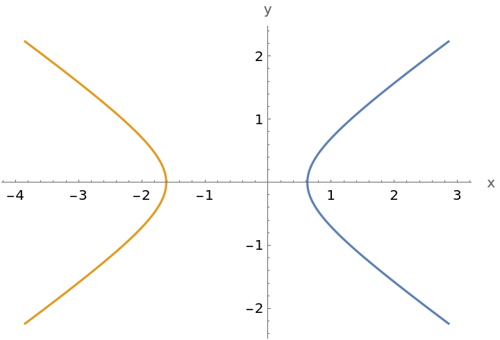
Function Repository Resource:

ConicSectionPlot

Source Notebook

Classifies and plots any polynomial of degree two or less in two or fewer variables

Contributed by: Dennis M Schneider and Robby S Villegas

ResourceFunction["ConicSectionPlot"][poly,vars]

plots the conic section specified by the expression poly=0 as a function of the variables vars.

ResourceFunction["ConicSectionPlot"][poly1poly2,vars]

returns ResourceFunction["ConicSectionPlot"][poly1-poly2,vars].

ResourceFunction["ConicSectionPlot"][poly,vars,"ReturnData"]

returns the data used to produce the plot, wrapped in Inactive.

Details and Options

The expression poly should be a polynomial of degree two or less, in two or fewer variables. The argument vars specifies the variables in poly, and must have length two.
With "ReturnData", the user has access to all the data used to produce the plot which allows the user make any desired modifications. Use Activate to restore the plot.
Styles for degenerate conics (a single point, a single line, two lines parallel or not) are set with the option "PrimitivesStyle".
ResourceFunction["ConicSectionPlot"] uses the resource function DiagonalizeQuadratic to compute the canonical form of a quadratic. Using the canonical form, it generates parametric equations of the curve.
The option "DrawAxes" allows for the principal axes to be included in the plot. The axes are color coded so that the axes colors Red and Green define a right-handed system. Other options are those of ParametricPlot.

Examples

Basic Examples (4) 

Plot a hyperbola:

In[1]:=
ResourceFunction["ConicSectionPlot"][x^2 - 2 y^2 + 3 + x - 4, {x, y}]
Out[1]=

Plot a rotated and translated hyperbola and show the axes:

In[2]:=
ResourceFunction["ConicSectionPlot"][
 x^2 + 3 y + 3 + x y + 2 x, {x, y}, "DrawAxes" -> True]
Out[2]=

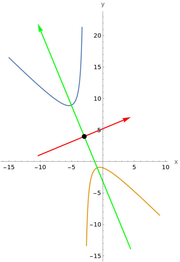
Plot a rotated and translated parabola and show the axes:
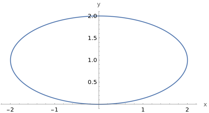
In[3]:=
ResourceFunction["ConicSectionPlot"][
 x^2 - 2 x y + y^2 + 2 x - y - 1, {x, y}, "DrawAxes" -> True]
Out[3]=

Plot an ellipse:

In[4]:=
ResourceFunction["ConicSectionPlot"][x^2 - 8 y + 4 y^2, {x, y}]
Out[4]=

Scope (10) 

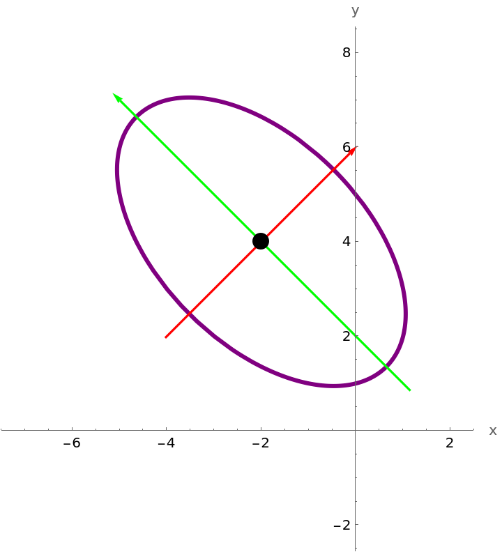
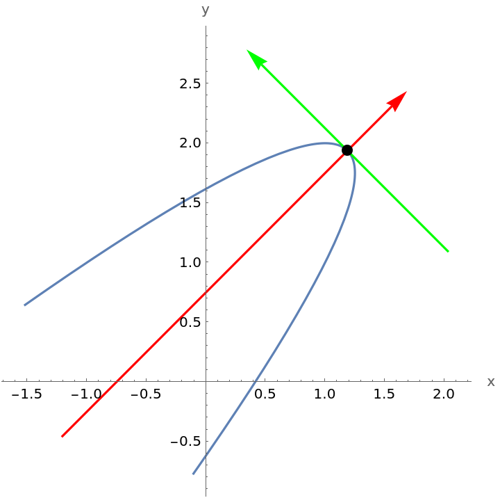
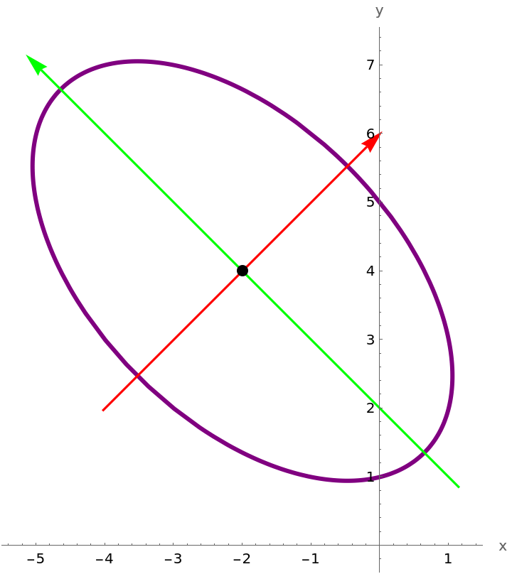
Plot a rotated and translated ellipse, with a style set for the ellipse, and show the axes:

In[5]:=
ResourceFunction["ConicSectionPlot"][
 5 + x^2 - 6 y + x y + y^2, {x, y}, PlotStyle -> {{AbsoluteThickness[3], Purple}}, "DrawAxes" -> True]
Out[5]=

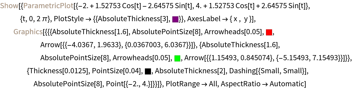
Use "ReturnData" to examine and possibly modify the data used to produce the plot and possibly modify the data:

In[6]:=
ellipse = ResourceFunction["ConicSectionPlot"][
  5 + x^2 - 6 y + x y + y^2, {x, y}, "ReturnData", PlotStyle -> {{AbsoluteThickness[3], Purple}}, "DrawAxes" -> True]
Out[6]=

Make several changes to the data (shrink the arrowheads, enlarge the center point, and enlarge the plot range) and plot the result:

In[7]:=
Inactive[Show][{Inactive[
     ParametricPlot][{-2.` + 1.5275252316519468` Cos[t] - 2.6457513110645903` Sin[t], 4.` + 1.5275252316519468` Cos[t] + 2.6457513110645903` Sin[t]}, {t, 0, 2 \[Pi]}, PlotStyle -> {{AbsoluteThickness[3], RGBColor[0.5, 0, 0.5]}}, AxesLabel -> {" x ", " y "}], Inactive[
     Graphics][{{{AbsoluteThickness[1.6`], AbsolutePointSize[8], Arrowheads[0.025], RGBColor[1, 0, 0], Arrow[{{-4.036700308869262`, 1.963299691130738`}, {0.0367003088692619`, 6.036700308869262`}}]}, {AbsoluteThickness[1.6`], AbsolutePointSize[8], Arrowheads[0.025], RGBColor[0, 1, 0], Arrow[{{1.1549263882819059`, 0.8450736117180941`}, {-5.154926388281906`, 7.154926388281906`}}]}}, {Thickness[0.0125`], PointSize[0.04`], GrayLevel[0], AbsoluteThickness[2], Dashing[{Small, Small}], AbsolutePointSize[12], Point[{-2.`, 4.`}]}}]}, PlotRange -> {{-7, 2}, {-2, 8}}, AspectRatio -> Automatic] // Activate
Out[7]=

Compare with the original plot:

In[8]:=
Activate[ellipse]
Out[8]=

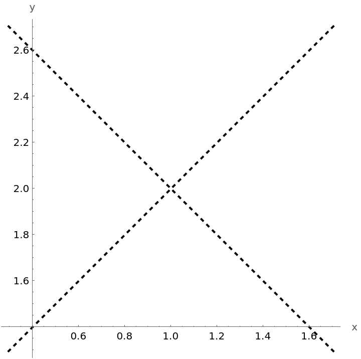
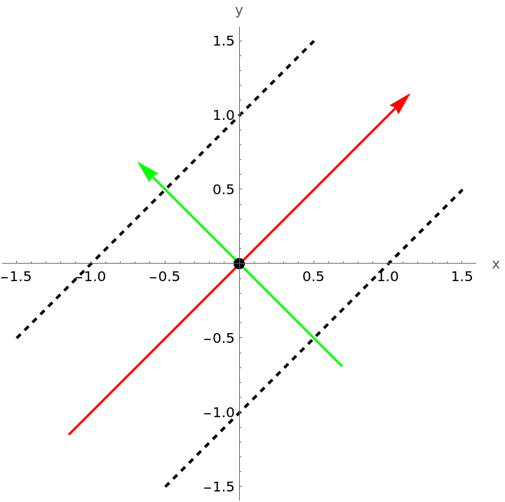
Plot a pair of intersecting lines:

In[9]:=
ResourceFunction[
 "ConicSectionPlot"][-3 - 2 x + x^2 + 4 y - y^2, {x, y}]
Out[9]=

These lines intersect because the polynomial can be expressed as a difference of squares. Confirm with the resource function CompleteTheSquare:

In[10]:=
ResourceFunction["CompleteTheSquare"][-3 - 2 x + x^2 + 4 y - y^2, {x, y}]
Out[10]=

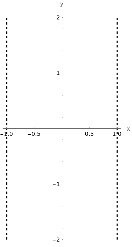
Plot a pair of parallel lines:

In[11]:=
ResourceFunction["ConicSectionPlot"][x^2 == 1, {x, y}]
Out[11]=

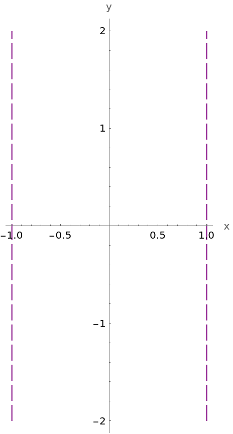
Change the style of the two lines using the option "PrimitivesStyle":

In[12]:=
ResourceFunction["ConicSectionPlot"][x^2 == 1, {x, y}, "PrimitivesStyle" -> {{Purple, Dashing[{Large, Small}]}}]
Out[12]=

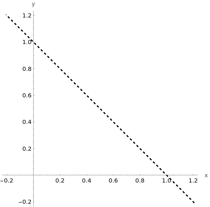
Plot an oblique line:

In[13]:=
ResourceFunction["ConicSectionPlot"][x + y == 1, {x, y}]
Out[13]=

Plot a pair of parallel oblique lines and show the axes:

In[14]:=
ResourceFunction["ConicSectionPlot"][(x - y)^2 == 1, {x, y}, "DrawAxes" -> True]
Out[14]=

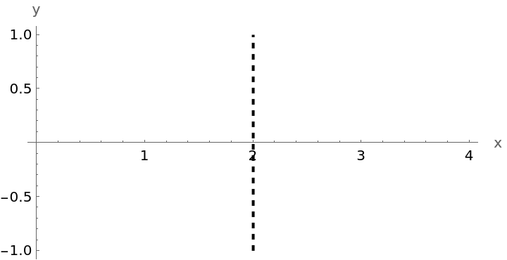
Plot a line parallel to a coordinate axis:

In[15]:=
ResourceFunction["ConicSectionPlot"][x - 2, {x, y}]
Out[15]=

This equation determines the whole plane:

In[16]:=
ResourceFunction["ConicSectionPlot"][x == x, {x, y}]
Out[16]=

This equation determines the empty set:

In[17]:=
ResourceFunction["ConicSectionPlot"][x^2 == -5, {x, y}]
Out[17]=

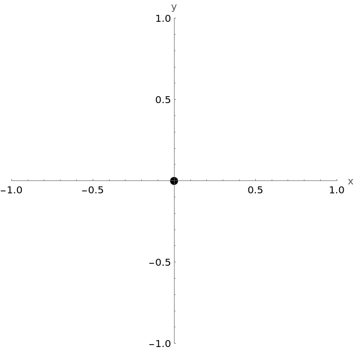
This equation determines the origin:

In[18]:=
ResourceFunction["ConicSectionPlot"][x^2 + y^2 == 0, {x, y}]
Out[18]=

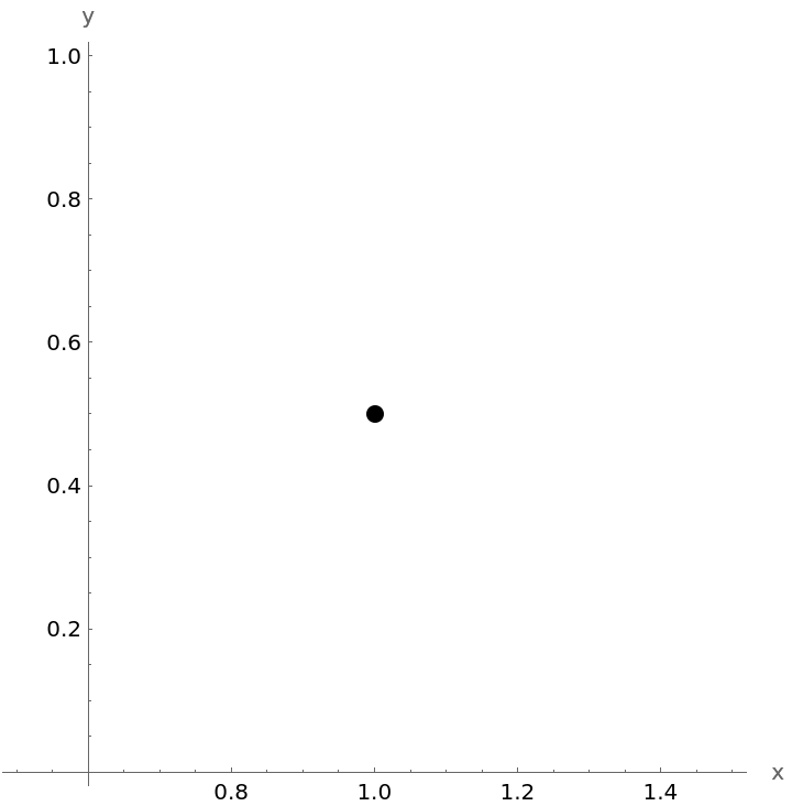
This equation determines point {1,1/2}:

In[19]:=
ResourceFunction["ConicSectionPlot"][(x - 1)^2 + (y - 1/2)^2, {x, y}]
Out[19]=

Possible Issues (4) 

ConicSectionPlot will returned $Failed if the degree of the quadratic is more than 2:

In[20]:=
ResourceFunction["ConicSectionPlot"][x^3 - y - 1, {x, y}]
Out[20]=

ConicSectionPlot will returned $Failed if the expression is not a polynomial:

In[21]:=
ResourceFunction["ConicSectionPlot"][Sin[x^3] - y - 1, {x, y}]
Out[21]=

ConicSectionPlot will returned $Failed if if there is not the correct number of input variables:

In[22]:=
ResourceFunction["ConicSectionPlot"][x^2 + y^2 - x y - 1, {x, y, z}]
Out[22]=

ConicSectionPlot will returned $Failed if the input expression is not a polynomial in the specified variables:

In[23]:=
ResourceFunction["ConicSectionPlot"][x^2 + y^2 - x y - 1, {x, u}]
Out[23]=

Publisher

Dennis M Schneider

Version History

  • 1.0.0 – 08 October 2019

Related Resources

License Information