Wolfram Function Repository
Instant-use add-on functions for the Wolfram Language
Function Repository Resource:
Visualize the behavior of conformal mappings in the complex plane
ResourceFunction["ComplexMapVisualization"][f] returns the ImageTransformation of a given function f on the complex plane. |
Visualize the sine function in the complex plane:
| In[1]:= |
| Out[1]= | 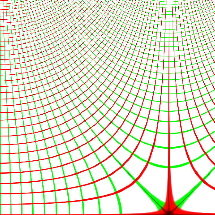 |
Mappings on different sections of the complex plane can be visualized by specifying a different DataRange or PlotRange:
| In[2]:= |
| Out[2]= | 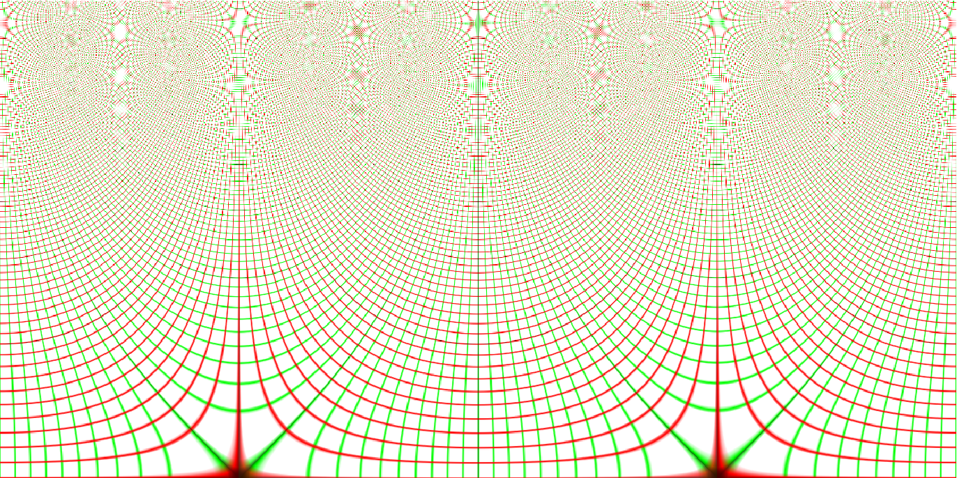 |
Forward transformations can be created by using the inverse function:
| In[3]:= |
| Out[3]= | 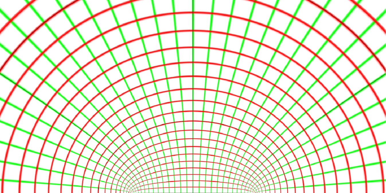 |
Standard special functions can be visualized:
| In[4]:= |
| Out[4]= | 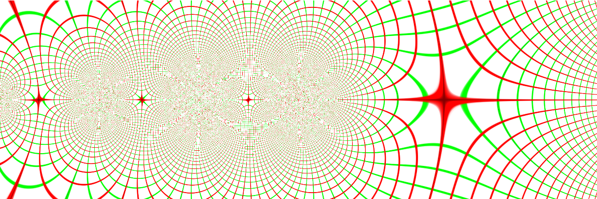 |
General functions that have complex values as their domain and range can be visualized:
| In[5]:= |
| Out[5]= | 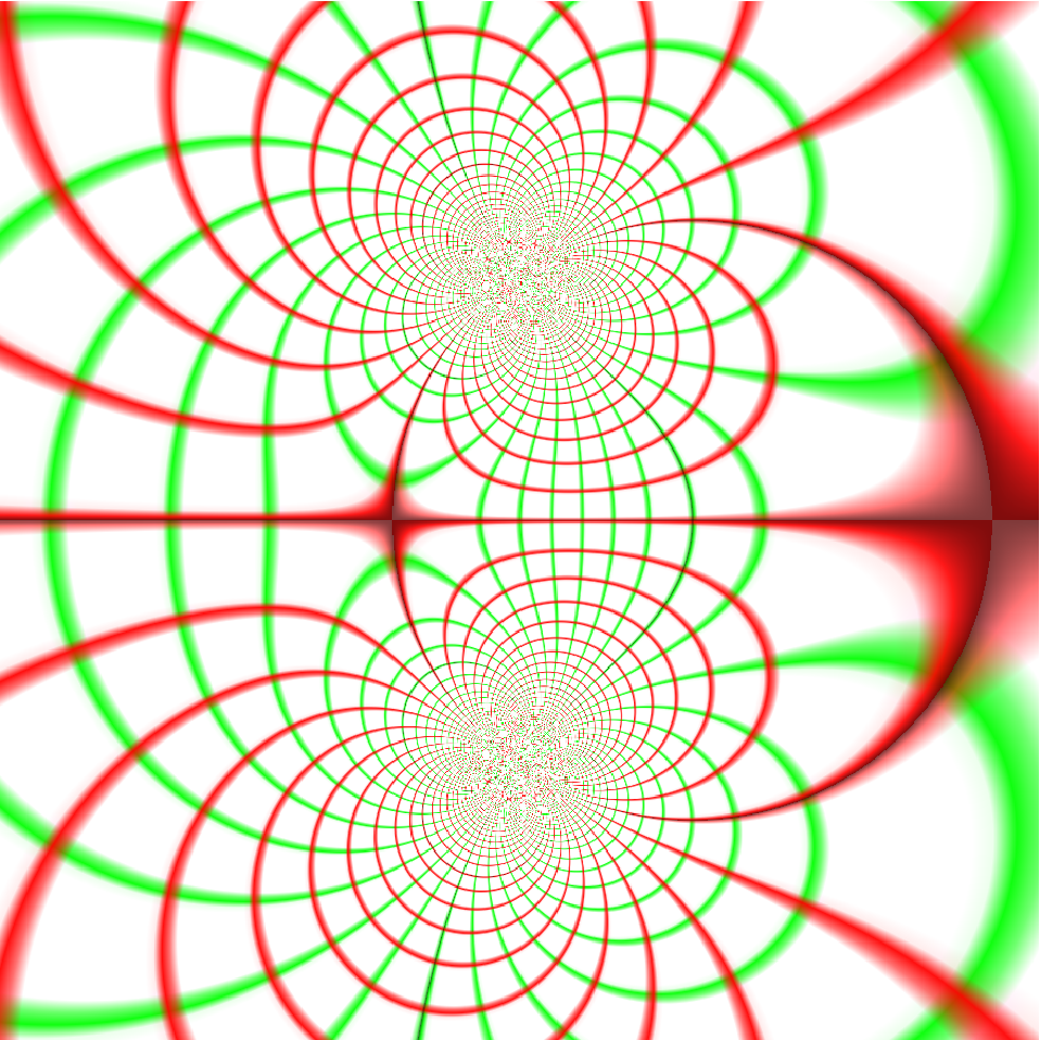 |
Compiled functions can be visualized:
| In[6]:= |
| Out[6]= |
| In[7]:= |
| Out[7]= | 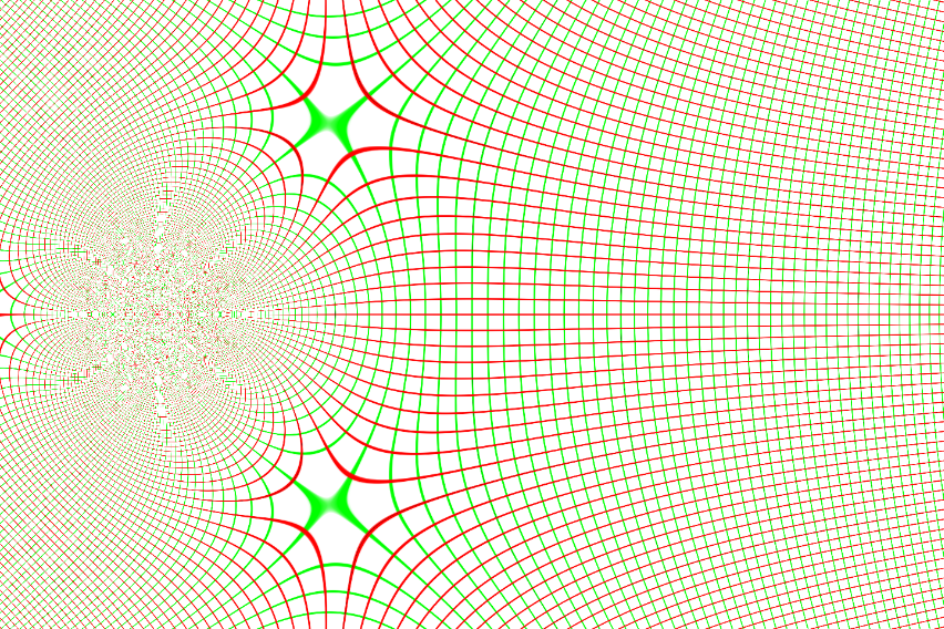 |
The "Image" option can be set to visualize mappings on arbitrary images or graphics objects:
| In[8]:= |
| Out[8]= | 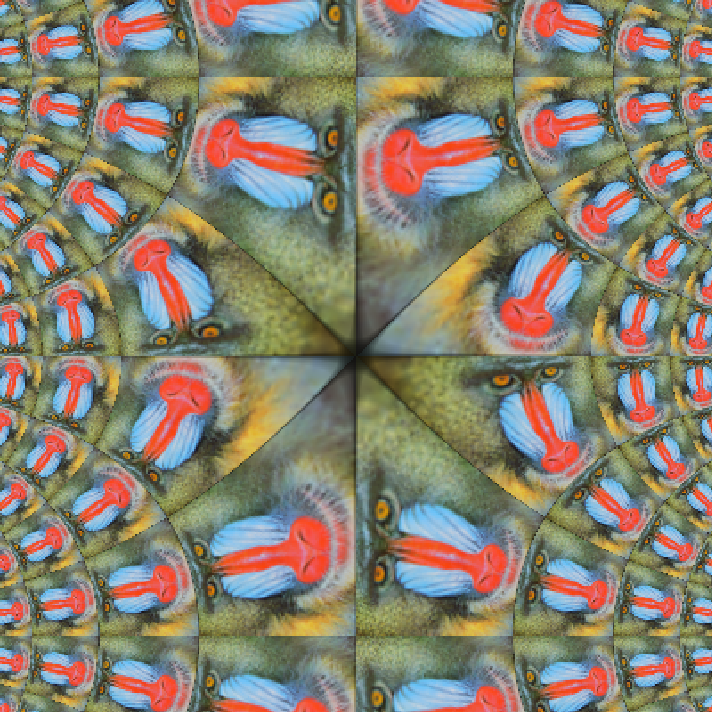 |
Use the "Image" option to see the transformation of a polar grid:
| In[9]:= | ![ResourceFunction["ComplexMapVisualization"][ProductLog, PlotRange -> {{-1, 1}, {-1, 1}}, "Image" -> \!\(\*
GraphicsBox[
{RGBColor[0, 1, 0], Thickness[0.01], CircleBox[{0, 0}, 0.], CircleBox[{0, 0}, 0.1], CircleBox[{0, 0}, 0.2], CircleBox[{0, 0}, 0.30000000000000004], CircleBox[{0, 0}, 0.4], CircleBox[{0, 0}, 0.5], CircleBox[{0, 0}, 0.6000000000000001], CircleBox[{0, 0}, 0.7000000000000001], CircleBox[{0, 0}, 0.8], CircleBox[{0, 0}, 0.9], CircleBox[{0, 0}, 1.], CircleBox[{0, 0}, 1.1], CircleBox[{0, 0}, 1.2000000000000002], CircleBox[{0, 0}, 1.3], CircleBox[{0, 0}, 1.4000000000000001],
{RGBColor[1, 0, 0],
TagBox[ConicHullRegionBox[{0, 0}, {{1, 0}}],
"InfiniteLine"],
TagBox[ConicHullRegionBox[{0, 0}, NCache[{{(Rational[
5, 8] + Rational[1, 8] 5^Rational[1, 2])^Rational[1, 2],
Rational[1, 4] (-1 + 5^Rational[1, 2])}}, {{
0.9510565162951535, 0.30901699437494745`}}]],
"InfiniteLine"],
TagBox[ConicHullRegionBox[{0, 0}, NCache[{{Rational[1, 4] (1 + 5^Rational[1, 2]), (
Rational[
5, 8] + Rational[-1, 8] 5^Rational[1, 2])^Rational[
1, 2]}}, {{0.8090169943749475, 0.5877852522924731}}]],
"InfiniteLine"],
TagBox[ConicHullRegionBox[{0, 0}, NCache[{{(Rational[
5, 8] + Rational[-1, 8] 5^Rational[1, 2])^Rational[
1, 2], Rational[1, 4] (1 + 5^Rational[1, 2])}}, {{
0.5877852522924731, 0.8090169943749475}}]],
"InfiniteLine"],
TagBox[ConicHullRegionBox[{0, 0}, NCache[{{Rational[1, 4] (-1 + 5^Rational[1, 2]), (
Rational[
5, 8] + Rational[1, 8] 5^Rational[1, 2])^Rational[
1, 2]}}, {{0.30901699437494745`, 0.9510565162951535}}]],
"InfiniteLine"],
TagBox[ConicHullRegionBox[{0, 0}, {{0, 1}}],
"InfiniteLine"],
TagBox[ConicHullRegionBox[{0, 0}, NCache[{{Rational[1, 4] (1 - 5^Rational[1, 2]), (
Rational[
5, 8] + Rational[1, 8] 5^Rational[1, 2])^Rational[
1, 2]}}, {{-0.30901699437494745`, 0.9510565162951535}}]],
"InfiniteLine"],
TagBox[ConicHullRegionBox[{0, 0}, NCache[{{-(Rational[
5, 8] + Rational[-1, 8] 5^Rational[1, 2])^Rational[
1, 2], Rational[1, 4] (
1 + 5^Rational[1, 2])}}, {{-0.5877852522924731, 0.8090169943749475}}]],
"InfiniteLine"],
TagBox[ConicHullRegionBox[{0, 0}, NCache[{{Rational[1, 4] (-1 - 5^Rational[1, 2]), (
Rational[
5, 8] + Rational[-1, 8] 5^Rational[1, 2])^Rational[
1, 2]}}, {{-0.8090169943749475, 0.5877852522924731}}]],
"InfiniteLine"],
TagBox[ConicHullRegionBox[{0, 0}, NCache[{{-(Rational[
5, 8] + Rational[1, 8] 5^Rational[1, 2])^Rational[
1, 2], Rational[
1, 4] (-1 + 5^Rational[1, 2])}}, {{-0.9510565162951535, 0.30901699437494745`}}]],
"InfiniteLine"],
TagBox[ConicHullRegionBox[{0, 0}, {{-1, 0}}],
"InfiniteLine"]}},
PlotRange->1]\)]](https://www.wolframcloud.com/obj/resourcesystem/images/eee/eeed6bd2-8f5a-4934-8427-f0f92cb749da/127e4ee90b2ada5e.png) |
| Out[9]= | 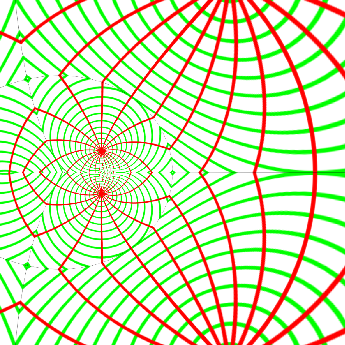 |
Options available to Rasterize affect the quality of the resulting image:
| In[10]:= |
| Out[10]= | 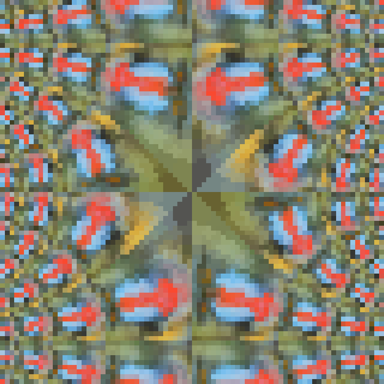 |
Using ParametricPlot on the inverse function gives a result similar to the one produced by ComplexMapVisualization:
| In[11]:= | ![With[{f = ArcSin}, {ResourceFunction["ComplexMapVisualization"][f, PlotRange -> {{-1, 1}, {-1, 1}}], ParametricPlot[
ReIm[InverseFunction[f][x + I y]], {x, -1, 1}, {y, -1, 1}, {BoundaryStyle -> None, ImageSize -> Large, Mesh -> Automatic, MeshStyle -> {
RGBColor[0, 1, 0],
RGBColor[1, 0, 0]}, PlotStyle -> GrayLevel[1]}]} // GraphicsRow]](https://www.wolframcloud.com/obj/resourcesystem/images/eee/eeed6bd2-8f5a-4934-8427-f0f92cb749da/43538522914651bb.png) |
| Out[11]= | 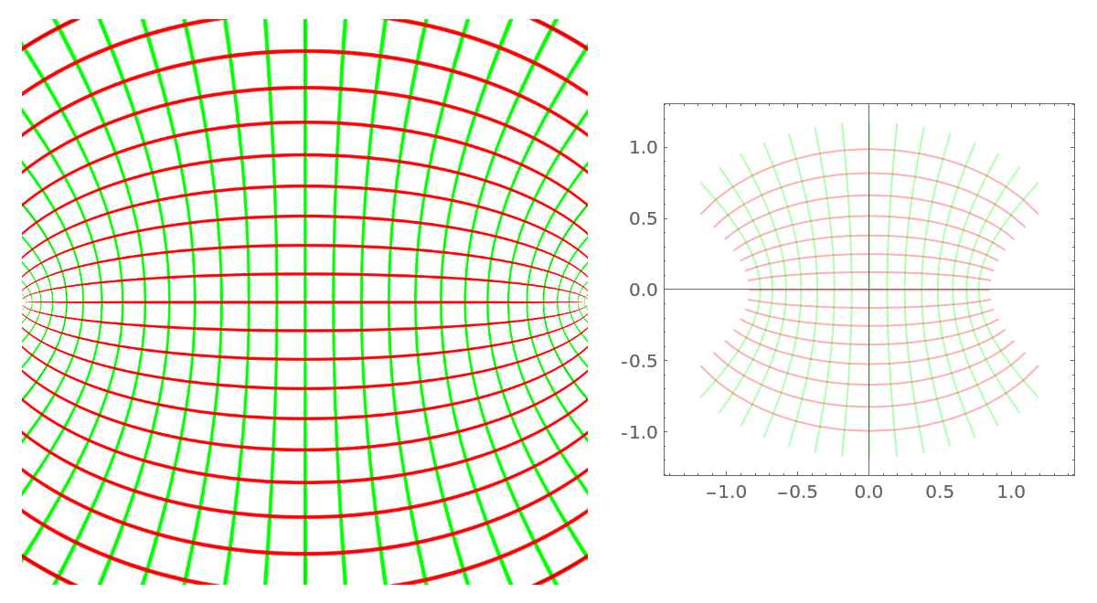 |
With a sufficiently large PlotRange, the computation may take a long time:
| In[12]:= |
| Out[12]= | 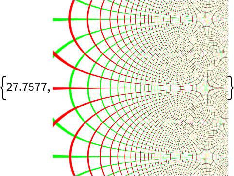 |
You can use the RasterSize option to reduce the quality of the input image and reduce the computation time:
| In[13]:= |
| Out[13]= | 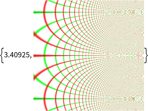 |
This work is licensed under a Creative Commons Attribution 4.0 International License