Basic Examples (2)
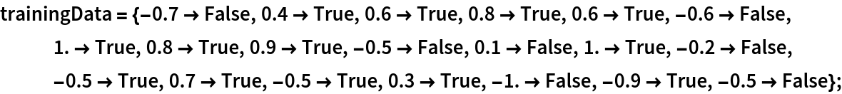
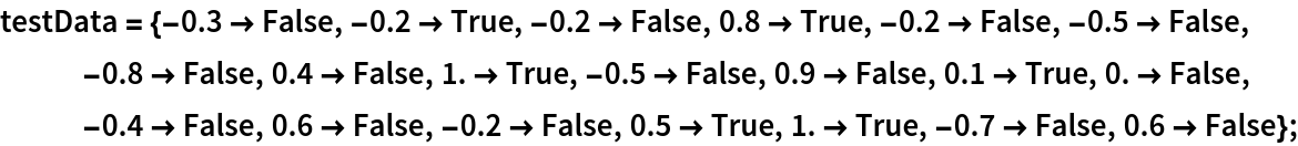
Get some simple training and test data:
Run a classifier and create a ClassifierMeasurementsObject:
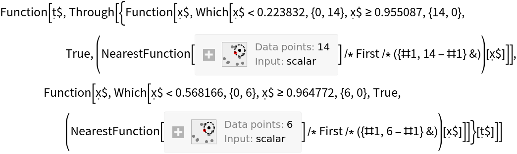
Create the ConfusionMatrixTrajectoryFunction:
Get the training and test sets of the Fisher iris data:
Create a classifier on the training set:
Construct a ClassifierMeasurementsObject from the classifier and the test set:
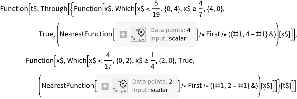
Construct a function that will, for any given probability threshold, construct the confusion matrix when "setosa" is designated as the positive class:
Apply that function to a threshold of 0.62 to get a confusion matrix:
Create a plot showing a trajectory of the false positive rate and true positive rate of the classifier for different thresholds:
Create a confusion matrix trajectory function as before, but let "virginica" be designated as the positive class:
Get the confusion matrix if the threshold is 0.62:
Scope (2)
One does not need a ClassifierMeasurementsObject to create the requisite function; the function will work with an Association that has the requisite key-value pairs as shown in the following example:
One can use the function on a neural network that has been converted to a classifier. Create a trained network following the method set forth here:
Create a ClassifierMeasurementsObject using testData:
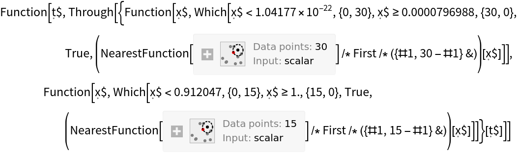
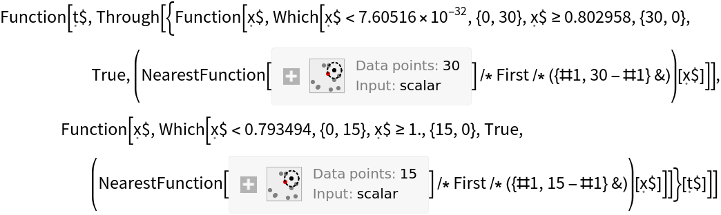
Create the confusion matrix trajectory function with "versicolor" as the positive class:
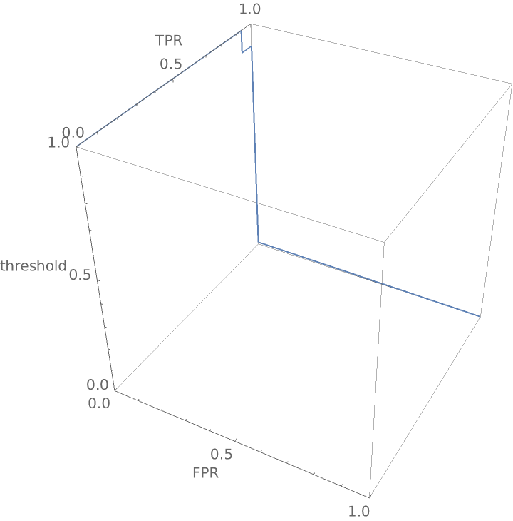
Show the three-dimensional ROC (receiver operating characteristic) curve for the network:
Applications (2)
Create functions that compute the false positive rate and true positive rate from a confusion matrix:
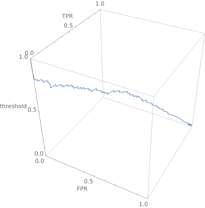
Construct a three-dimensional receiver operating curve that shows the false positive rate and true positive rate for "good" wine as a function of the threshold probability required before the classifier calls a wine "good":
Construct a ClassifierMeasurementsObject from the classifier and the test set:
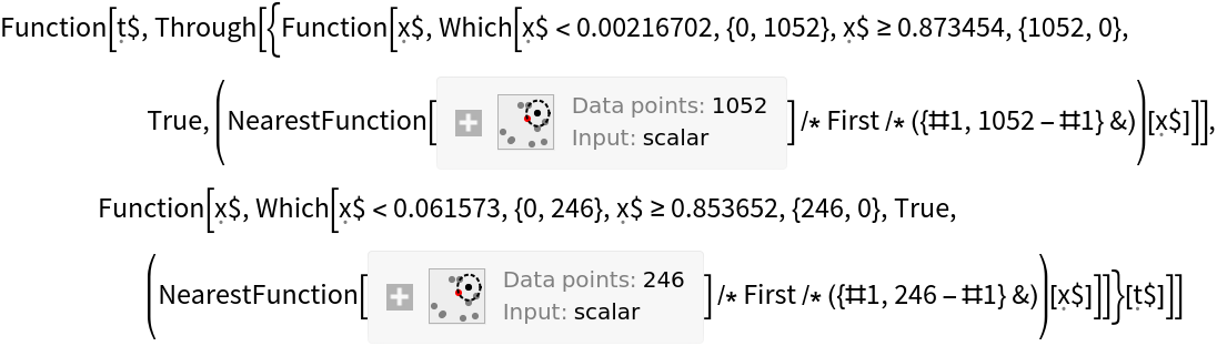
Create the confusion matrix function:
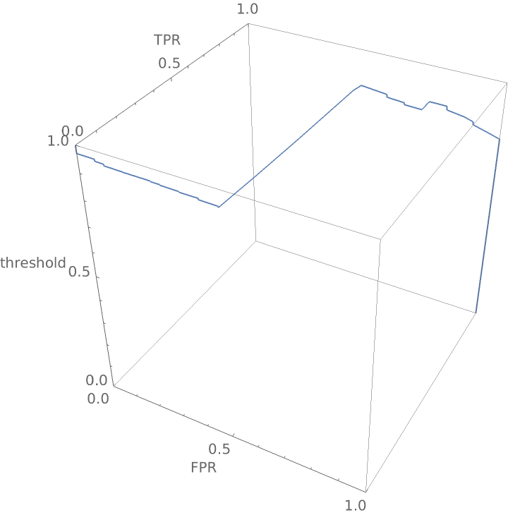
Create a three-dimensional plot:
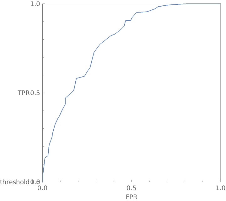
View the graphic from the top as a traditional receiver operating curve:
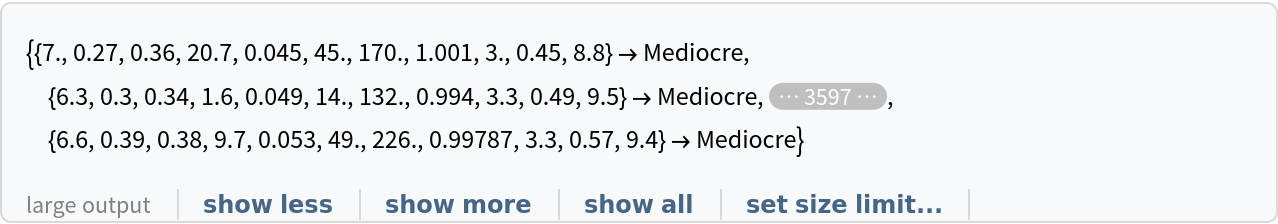
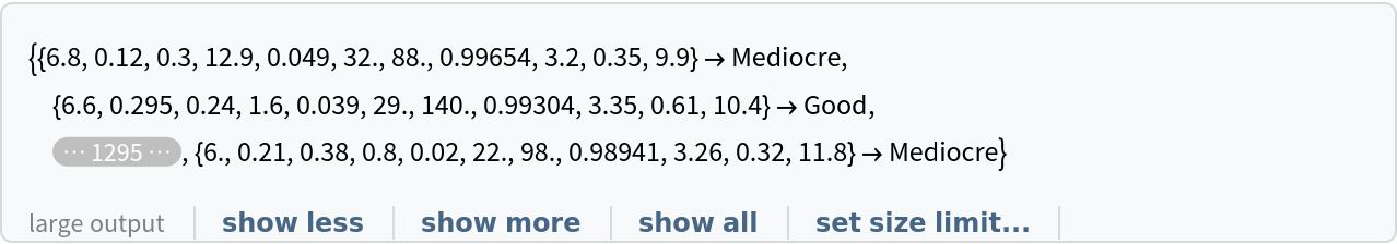
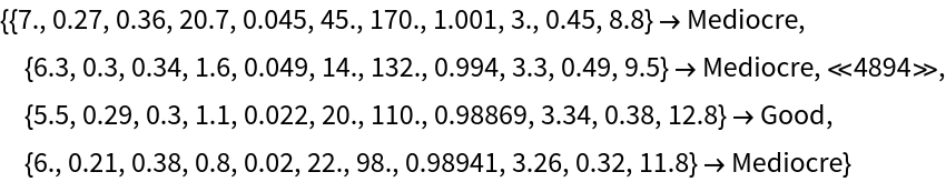
The function works well in conjunction with the CrossValidateModel resource function and permits one to smooth the confusion matrix trajectory. Start this process by creating a query that will convert continuous wine quality values into discrete bins of Good, Bad and Mediocre:
Create wine data suitable for Classify:
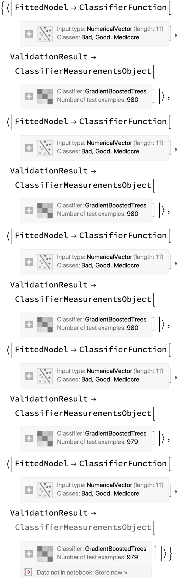
Run the CrossValidateModel resource function to create five pairs of ClassifierFunction and ClassifierMeasurementsObject for each of the five folds:
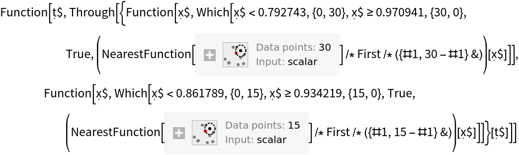
Create confusion matrix trajectory functions for each of the five folds:
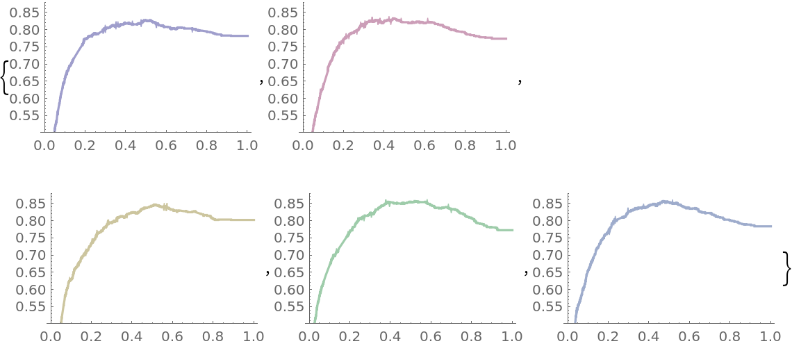
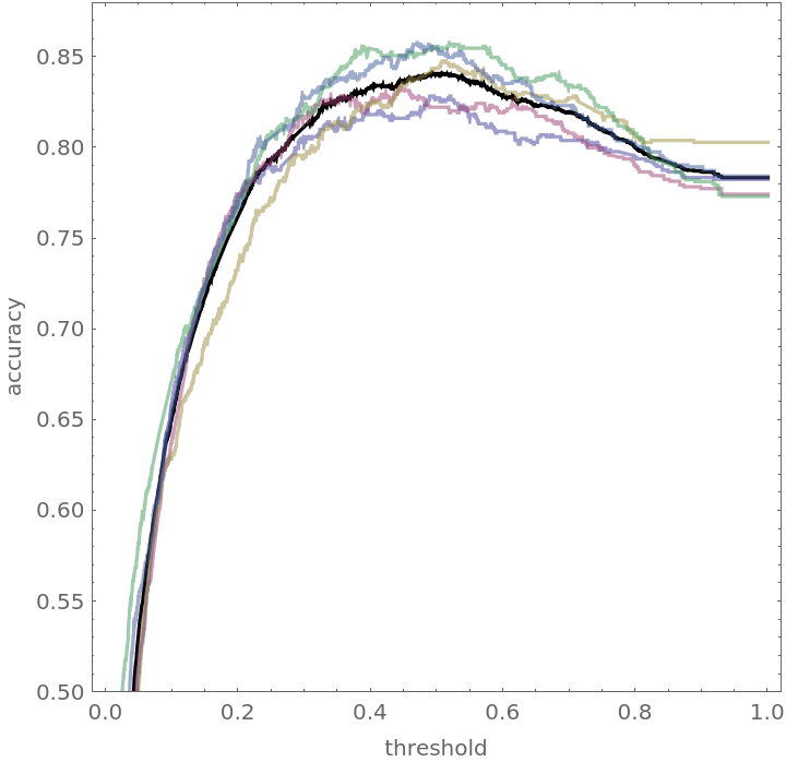
Plot the accuracy of the classifier over the threshold levels for each of the folds:
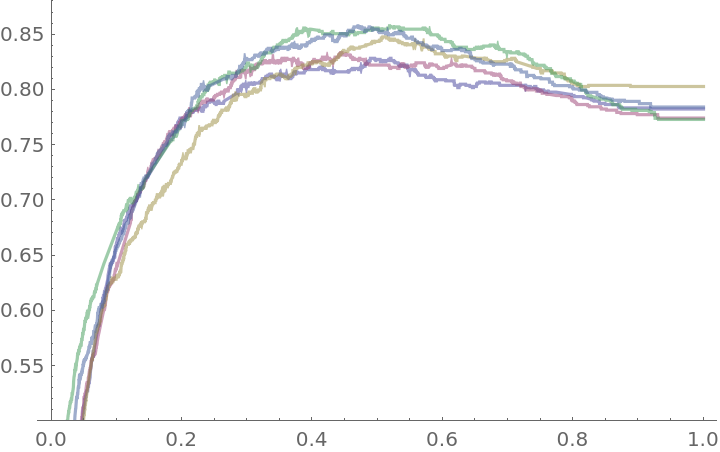
Create a composite view of the five accuracy plots:
Now create a function that computes confusion matrices for all five folds:
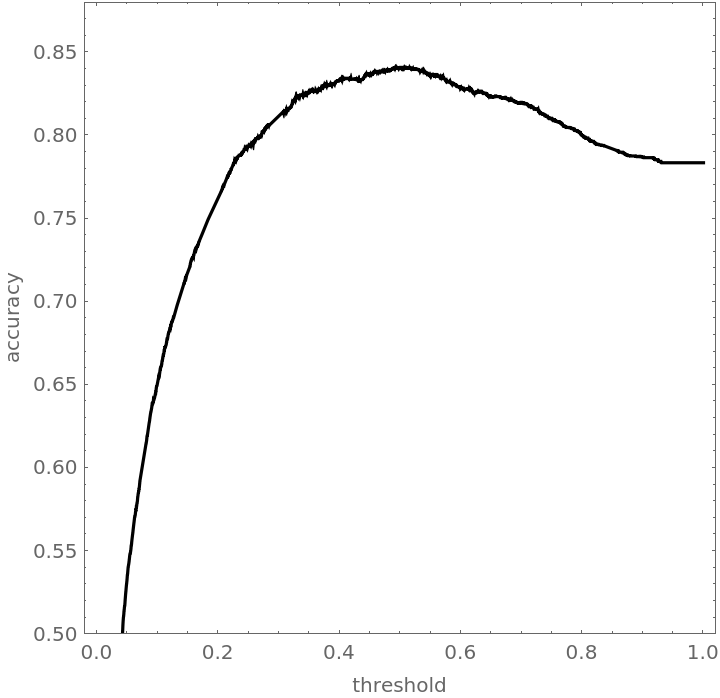
Plot the blended accuracy curve:
Show the blended accuracy plot and the components creating it:
Neat Examples (4)
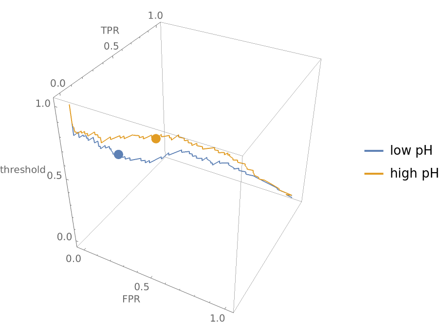
Compare how a classifier performs on wines with low pH versus wines with high pH:
Show the three-dimensional ROC curves and draw points where the threshold is 0.5:
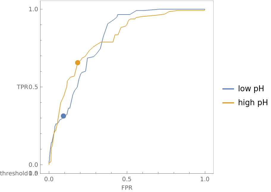
Show the graphic from the top and notice that even though the ROC curves look roughly the same in two dimensions, the false positive and true positive rates for the two different pH groupings of wine differ significantly at a threshold of 0.5:
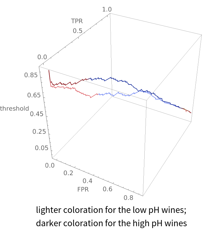
Create the same plot but make the hue of each plot line depend on the accuracy of the classifier at that threshold:
![falsePositiveRate[cm : {{tn_, fp_}, {fn_, tp_}}] := fp/(tn + fp);
truePositiveRate[cm : {{tn_, fp_}, {fn_, tp_}}] := tp/(fn + tp)](https://www.wolframcloud.com/obj/resourcesystem/images/9cf/9cf5d13a-ef16-4f66-9e1f-872bcd91edc3/374a4fb2cc6eaa38.png)
![cmfSimple = ResourceFunction[
"ConfusionMatrixTrajectoryFunction"][<|"LogProbabilities" -> {{-Log[
7], -Log[7/4], -Log[7/2]}, {-Log[12/7], -Log[4], -Log[
6]}, {-Log[7/3], -Log[7/2], -Log[7/2]}, {-Log[9/5], -Log[
3], -Log[9]}, {-Log[19/6], -Log[19/5], -Log[19/8]}, {-Log[17/
3], -Log[17/4], -Log[17/10]}}, "TestSet" -> <|"Output" -> {"virginica", "versicolor", "setosa", "virginica", "setosa", "versicolor"}|>, "ExtendedClasses" -> {"setosa", "versicolor", "virginica"}|>, "versicolor"]](https://www.wolframcloud.com/obj/resourcesystem/images/9cf/9cf5d13a-ef16-4f66-9e1f-872bcd91edc3/0cbe8efd72d7ed20.png)
![trainingData = ExampleData[{"MachineLearning", "FisherIris"}, "TrainingData"];
testData = ExampleData[{"MachineLearning", "FisherIris"}, "TestData"];
labels = Union[Values[trainingData]];
net = NetChain[{3, SoftmaxLayer[]}, "Input" -> 4, "Output" -> NetDecoder[{"Class", labels}]];
results = NetTrain[net, trainingData, All, MaxTrainingRounds -> 100];
trained = results["TrainedNet"];
clNet = Classify[trained]](https://www.wolframcloud.com/obj/resourcesystem/images/9cf/9cf5d13a-ef16-4f66-9e1f-872bcd91edc3/4cd2769caf0f0168.png)
![falsePositiveRate[cm : {{tn_, fp_}, {fn_, tp_}}] := fp/(tn + fp);
truePositiveRate[cm : {{tn_, fp_}, {fn_, tp_}}] := tp/(fn + tp)](https://www.wolframcloud.com/obj/resourcesystem/images/9cf/9cf5d13a-ef16-4f66-9e1f-872bcd91edc3/4aba39900556b6a2.png)
![binWine = Query[All, ReplacePart[#, 2 -> Which[#[[2]] >= 7, "Good", #[[2]] < 5, "Bad", True, "Mediocre"]] &];](https://www.wolframcloud.com/obj/resourcesystem/images/9cf/9cf5d13a-ef16-4f66-9e1f-872bcd91edc3/04dc9d194a003a7f.png)
![ParametricPlot3D[
Append[Through[{falsePositiveRate, truePositiveRate}[cmfWine[t]]], t], {t, 0, 1}, AxesLabel -> {"FPR", "TPR", "threshold"}, BoxRatios -> {1, 1, 1}, PlotRange -> {{0, 1}, {0, 1}, {0, 1}}]](https://www.wolframcloud.com/obj/resourcesystem/images/9cf/9cf5d13a-ef16-4f66-9e1f-872bcd91edc3/1529b1d6059fc830.png)
![binWine = Query[All, ReplacePart[#, 2 -> Which[#[[2]] >= 7, "Good", #[[2]] < 5, "Bad", True, "Mediocre"]] &];](https://www.wolframcloud.com/obj/resourcesystem/images/9cf/9cf5d13a-ef16-4f66-9e1f-872bcd91edc3/4f82de2820c6a327.png)
![(wineCMTrajectories = Query[All, "ValidationResult" /* (ResourceFunction[
"ConfusionMatrixTrajectoryFunction"][#, "Good"] &)][
crossValidatedWine]) // Shallow[#, 5] &](https://www.wolframcloud.com/obj/resourcesystem/images/9cf/9cf5d13a-ef16-4f66-9e1f-872bcd91edc3/2370e00b67c6509f.png)
![wineAccuracyPlots = MapIndexed[
Plot[accuracy[#[t]], {t, 0, 1}, PlotRange -> {0.5, 0.88}, PlotStyle -> {Opacity[0.5], ColorData[1][#2[[1]]]}] &, wineCMTrajectories]](https://www.wolframcloud.com/obj/resourcesystem/images/9cf/9cf5d13a-ef16-4f66-9e1f-872bcd91edc3/06bb9753aee1e607.png)
![blendedWineAccuracyPlot = Plot[With[{cm = Mean[blendedWineTrajectory[t]]}, accuracy[cm]], {t, 0, 1}, PlotRange -> {0.5, 0.88}, PlotStyle -> Black, AspectRatio -> 1, Frame -> True, FrameLabel -> {"threshold", "accuracy"}]](https://www.wolframcloud.com/obj/resourcesystem/images/9cf/9cf5d13a-ef16-4f66-9e1f-872bcd91edc3/2095c318554c3d14.png)
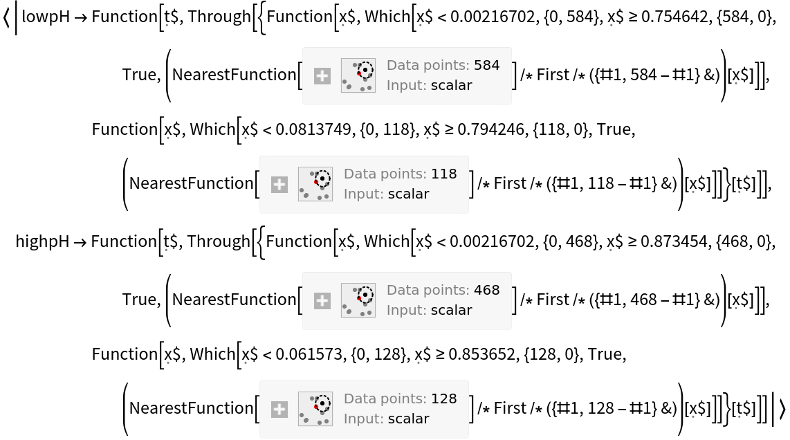
![confusionMatrixFunctionsBypH = KeyTake[{"lowpH", "highpH"}][ResourceFunction[
ResourceObject[
Association[
"Name" -> "MapReduceOperator", "ShortName" -> "MapReduceOperator", "UUID" -> "856f4937-9a4c-44a9-88ae-cfc2efd4698f", "ResourceType" -> "Function", "Version" -> "1.0.0", "Description" -> "Like an operator form of GroupBy, but where \
one also specifies a reducer function to be applied", "RepositoryLocation" -> URL[
"https://www.wolframcloud.com/objects/resourcesystem/api/1.0"]\
, "SymbolName" -> "FunctionRepository`$\
ad7fe533436b4f8294edfa758a34ac26`MapReduceOperator", "FunctionLocation" -> CloudObject[
"https://www.wolframcloud.com/obj/6d981522-1eb3-4b54-84f6-\
55667fb2e236"]], ResourceSystemBase -> Automatic]][
If[#[[1, 9]] < 3.18, "lowpH", "highpH"] &, (ClassifierMeasurements[
cWine, #] &) /* (ResourceFunction[
"ConfusionMatrixTrajectoryFunction"][#, "Good"] &)][
wineTestData]]](https://www.wolframcloud.com/obj/resourcesystem/images/9cf/9cf5d13a-ef16-4f66-9e1f-872bcd91edc3/6b0a83582361d702.png)
![With[{low = confusionMatrixFunctionsBypH["lowpH"], high = confusionMatrixFunctionsBypH["highpH"]},
Show[ParametricPlot3D[{Append[
Through[{falsePositiveRate, truePositiveRate}[low[t]]], t], Append[Through[{falsePositiveRate, truePositiveRate}[high[t]]], t]}, {t, 0, 1}, AxesLabel -> {"FPR", "TPR", "threshold"}, PlotLegends -> {"low pH", "high pH"}], Graphics3D[{PointSize[0.03], RGBColor[0.368417, 0.506779, 0.709798],
Point[Append[
Through[{falsePositiveRate, truePositiveRate}[low[0.5]]], 0.5]],
RGBColor[0.880722, 0.611041, 0.142051], Point[Append[
Through[{falsePositiveRate, truePositiveRate}[high[0.5]]], 0.5]]}]]
]](https://www.wolframcloud.com/obj/resourcesystem/images/9cf/9cf5d13a-ef16-4f66-9e1f-872bcd91edc3/49da988f350d83ae.png)
![With[{low = confusionMatrixFunctionsBypH["lowpH"], high = confusionMatrixFunctionsBypH["highpH"]}, Module[{lowplot = ParametricPlot3D[{Append[
Through[{falsePositiveRate, truePositiveRate}[low[t]]], t]}, {t, 0.1, 0.9}, AxesLabel -> {"FPR", "TPR", "threshold"}, ColorFunctionScaling -> True, ColorFunction -> (With[{i = With[{m = low[#3]}, Total[m[[2]]]/Total[m, 2]]}, Lighter@ColorData[
"TemperatureMap"][((-1 + i) (-1 + #1) + (-2 + i + 2 #1) #2)/Max[0.01, #1 - #2]]] &)],
highplot = ParametricPlot3D[{Append[
Through[{falsePositiveRate, truePositiveRate}[high[t]]], t]}, {t, 0.1, 0.9}, AxesLabel -> {"FPR", "TPR", "threshold"}, ColorFunctionScaling -> True, ColorFunction -> (With[{i = With[{m = high[#3]}, Total[m[[2]]]/Total[m, 2]]}, Darker@ColorData[
"TemperatureMap"][((-1 + i) (-1 + #1) + (-2 + i + 2 #1) #2)/Max[0.01, #1 - #2]]] &)]},
Labeled[Show[lowplot, highplot], Style["lighter coloration for the low pH wines;\ndarker coloration \
for the high pH wines", "Text"]]
]
]](https://www.wolframcloud.com/obj/resourcesystem/images/9cf/9cf5d13a-ef16-4f66-9e1f-872bcd91edc3/272cc3b2b6da987a.png)