Wolfram Function Repository
Instant-use add-on functions for the Wolfram Language
Function Repository Resource:
Alter a confusion matrix by stochastically flipping classification results
ResourceFunction["ConfusionMatrixFlip"][m,r] flips a matrix m using a matrix r in which rij represents the fraction of instances for which an instance in column i will flip into column j. | |
ResourceFunction["ConfusionMatrixFlip"][m,flips] flips a 2×2 matrix using a vector to give the proportions of flips between columns. |
Flip a 2×2 confusion matrix by randomly reversing 20% of the instances classified as negative and 40% of the instances classified as positive:
| In[1]:= |
|
| Out[1]= |
|
Use a simplified syntax to accomplish the same flip :
| In[2]:= |
|
| Out[2]= |
|
Flip a 3 ×3 matrix by moving 30% of those classified as 1 to 2 and 10% of those classified as 1 to 3; by moving 0% of those classified as 2 to 1 and 40% of those classified as 2 to 3; and by moving 50% of those classified as 3 to 2 and 10% of those classified as 3 to 1:
| In[3]:= |
|
| Out[3]= |
|
Both the confusion matrix and the flip matrix can be symbolic:
| In[4]:= |
|
| Out[4]= |
|
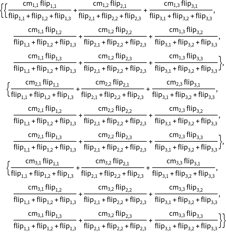
Find out how much the accuracy of a classifier declines using a symbolic confusion matrix and symbolic set of flips:
| In[5]:= |
![Collect[Simplify@
Module[{m = Array[Subscript[cm, ##] &, {2, 2}], originalAccuracy, flippedAccuracy}, originalAccuracy = Total@Diagonal[m]/Total[m, 2];
flippedAccuracy = 1/Total[m, 2] Total@
Diagonal[
ResourceFunction["ConfusionMatrixFlip"][m, {flipneg, flippos}]];
1 - flippedAccuracy/originalAccuracy], {flipneg, flippos}]](https://www.wolframcloud.com/obj/resourcesystem/images/717/717f7f65-9333-45b9-9752-fa5a681cf49f/3bb7a9b3a499f7a1.png)
|
| Out[5]= |
|
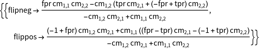
Given an original 2×2 confusion matrix, find the set of flips such that the false positive rate and true positive rate equal some pair {fpr,tpr}:
| In[6]:= |
![With[{flipped = ResourceFunction["ConfusionMatrixFlip"][
Array[Subscript[cm, ##] &, {2, 2}], {flipneg, flippos}]}, Solve[{flipped[[1, 2]]/Total[flipped[[1]]] == fpr, flipped[[2, 2]]/Total[flipped[[2]]] == tpr}, {flipneg, flippos}]] // FullSimplify](https://www.wolframcloud.com/obj/resourcesystem/images/717/717f7f65-9333-45b9-9752-fa5a681cf49f/4f6dc48d29c7c50f.png)
|
| Out[6]= |
|
Given an original 2×2 confusion matrix, find the set of flips such that the positive classification rate equals some value pcr:
| In[7]:= |
![With[{flipped = ResourceFunction["ConfusionMatrixFlip"][
Array[Subscript[cm, ##] &, {2, 2}], {flipneg, flippos}]}, Quiet[Solve[{(flipped[[1, 2]] + flipped[[2, 2]])/
Total[flipped, 2] == pcr}, {flipneg, flippos}]]] // FullSimplify](https://www.wolframcloud.com/obj/resourcesystem/images/717/717f7f65-9333-45b9-9752-fa5a681cf49f/0454a0d4aaadf682.png)
|
| Out[7]= |
|
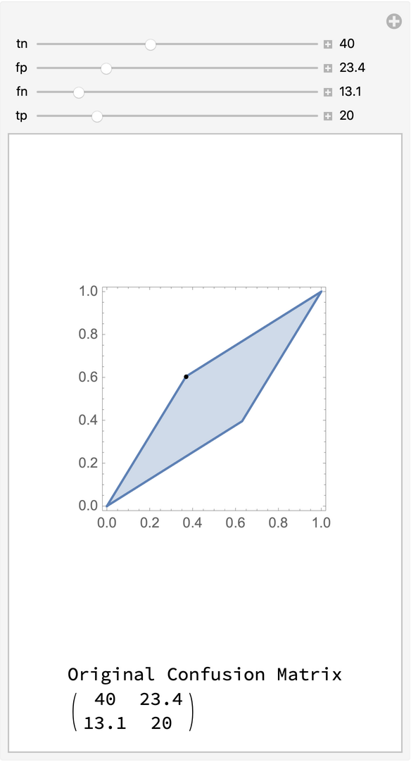
Show the set of possible false positive rates and true positive rates attainable by flipping a confusion matrix derived from a classifier:
| In[8]:= |
![Manipulate[Module[{cm = {{tn, fp}, {fn, tp}}, flipped, fpr, tpr},
Labeled[
RegionPlot[
0 <= (fpr (cm[[1, 1]] + cm[[1, 2]]) cm[[2, 2]] - tpr cm[[1, 2]] (cm[[2, 1]] + cm[[2, 2]]))/(-cm[[1, 2]] cm[[2,
1]] + cm[[1, 1]] cm[[2, 2]]) <= 1 && 0 <= ((tpr cm[[1, 1]] + cm[[1, 2]] - fpr (cm[[1, 1]] + cm[[1, 2]])) cm[[2, 1]] + (-1 + tpr) cm[[1, 1]] cm[[2, 2]])/(cm[[1, 2]] cm[[2, 1]] - cm[[1, 1]] cm[[2, 2]]) <= 1, {fpr, 0, 1}, {tpr, 0, 1}, Epilog -> {PointSize[0.02], Point[{fp/(fp + tn), tp/(tp + fn)}]}],
Column[{"Original Confusion Matrix", MatrixForm[{{tn, fp}, {fn, tp}}]}]]
],
{{tn, 40}, 0.1, 100, Appearance -> "Labeled"},
{{fp, 30}, 0.1, 100, Appearance -> "Labeled"},
{{fn, 10}, 0.1, 100, Appearance -> "Labeled"},
{{tp, 20}, 0.1, 100, Appearance -> "Labeled"}]](https://www.wolframcloud.com/obj/resourcesystem/images/717/717f7f65-9333-45b9-9752-fa5a681cf49f/0b8708cf8c5c9077.png)
|
| Out[8]= |
|
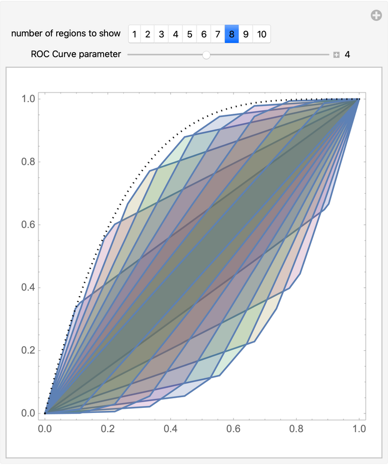
Approximate the region of attainable false positive and true positive rates given a receiver operating characteristic curve (shown as a dotted line) and a set of flips:
| In[9]:= |
![Manipulate[
Show @@ Append[
MapIndexed[{f, index} |-> With[{att = attainable[f, CDF[BetaDistribution[1, rocvalue]], 0.5]},
RegionPlot[att[fpr, tpr], {fpr, 0, 1}, {tpr, 0, 1}, PlotStyle -> {Opacity[0.2], ColorData[1][index[[1]]]}]
], Subdivide[0.1, 0.9, n]], Plot[CDF[BetaDistribution[1, rocvalue], f], {f, 0, 1}, PlotStyle -> Directive[{Dotted, Black}]]],
{{n, 8, "number of regions to show"}, Range[10], ControlType -> SetterBar},
{{rocvalue, 4, "ROC Curve parameter"}, 1.5, 8, 0.1, Appearance -> "Labeled"},
Initialization :> (attainable[cm_] = Function[{fpr, tpr}, 0 <= (fpr (cm[[1, 1]] + cm[[1, 2]]) cm[[2, 2]] - tpr cm[[1, 2]] (cm[[2, 1]] + cm[[2, 2]]))/(-cm[[1, 2]] cm[[
2, 1]] + cm[[1, 1]] cm[[2, 2]]) <= 1 && 0 <= ((tpr cm[[1, 1]] + cm[[1, 2]] - fpr (cm[[1, 1]] + cm[[1, 2]])) cm[[2, 1]] + (-1 + tpr) cm[[1, 1]] cm[[2, 2]])/(cm[[1, 2]] cm[[2,
1]] - cm[[1, 1]] cm[[2, 2]]) <= 1]; attainable[fpr_, tprfunc_, i_] := attainable[{{1 - fpr - i + fpr i, fpr - fpr i}, {i - i tprfunc[fpr], i tprfunc[fpr]}}])]](https://www.wolframcloud.com/obj/resourcesystem/images/717/717f7f65-9333-45b9-9752-fa5a681cf49f/5358c588fa423d20.png)
|
| Out[9]= |
|
This work is licensed under a Creative Commons Attribution 4.0 International License