Details and Options
The recognized formats for
data are listed in the left-hand column below. The right-hand column shows examples of symbols that take the same data format. Note that
Dataset is currently not supported.
| List: {…} | EstimatedDistribution,LinearModelFit,GeneralizedLinearModelFit,NonlinearModelFit,Predict,Classify,NetTrain,SpatialEstimate |
| Rule of lists: {…}→ {…} | Predict,Classify,NetTrain,SpatialEstimate |
| Association of lists: <|key1→ {…},…|> | NetTrain |
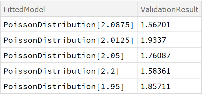
ResourceFunction["CrossValidateModel"] divides the data repeatedly into randomly chosen training and validation sets. Each time, fitfun is applied to the training set. The returned model is then validated against the validation set. The returned result is of the form {<|"FittedModel"→ model1, "ValidationResult" → result1|>, …}.
For any distribution that satisfies
DistributionParameterQ, the syntax for fitting distributions is the same as for
EstimatedDistribution, which is the function that is being used internally to fit the data. The returned values of
EstimatedDistribution are found under the
"FittedModel" keys of the output. The
"ValidationResult" lists the average negative
LogLikelihood on the validation set, which is the default loss function for distribution fits.
If the user does not specify a validation function explicitly using the "ValidationFunction" option, ResourceFunction["CrossValidateModel"] tries to automatically apply a sensible validation loss metric for results returned by fitfun (see the next table). If no usable validation method is found, the validation set itself will be returned so that the user can perform their own validation afterward.
The following table lists the types of models that are recognized, the functions that produce such models and the default loss function applied to that type of model:
An explicit validation function can be provided with the
"ValidationFunction" option. This function takes the fit result as a first argument and a validation set as a second argument. If multiple models are specified as an
Association in the second argument of
ResourceFunction["CrossValidateModel"], different validation functions for each model can be specified by passing an
Association to the
"ValidationFunction" option.
The
Method option can be used to configure how the training and validation sets are generated. The following types of sampling are supported:
| "KFold" (default) | splits the dataset into k subsets (default: k=5) and trains the model k times, using each partition as validation set once |
| "LeaveOneOut" | fit the data as many times as there are elements in the dataset, using each element for validation once |
| "RandomSubSampling" | split the dataset randomly into training and validation sets (default: 80% / 20%) repeatedly (default: five times) or define a custom sampling function |
| "BootStrap" | use bootstrap samples (generated with RandomChoice) to fit the model repeatedly without validation |
The default
Method setting uses
k-fold validation with five folds. This means that the dataset is randomly split into five partitions, where each is used as the validation set once. This means that the data gets trained five times on 4/5 of the dataset and then tested on the remaining 1/5. The
"KFold" method has two sub-options:
| "Folds" | 5 | number of partitions in which to split the dataset |
| "Runs" | 1 | number of times to perform k-fold validation (each time with a new random partitioning of the data) |
The
"LeaveOneOut" method, also known as the jackknife method, is essentially
k-fold validation where the number of folds is equal to the number of data points. Since it can be quite computationally expensive, it is usually a good idea to use parallelization with this method. It does have the
"Runs" sub-option like the
"KFold" method, but for deterministic fitting procedures like
EstimatedDistribution and
LinearModelFit, there is no value in performing more than one run since each run will yield the exact same results (up to a random permutation).
The method "RandomSubSampling" splits the dataset into training/validation sets randomly and has the following sub-options:
| "Runs" | 1 | number of times to resample the data into training/validation sets |
| ValidationSet | Scaled[1/5] | number of samples to use for validation. When specified as Scaled[f], a fraction f of the dataset will be used for validation |
| "SamplingFunction" | Automatic | function that specifies how to sub-sample the data |
For the option
"SamplingFunction", the function
fun[nData,nVal] should return an
Association with the keys "TrainingSet" and "ValidationSet". Each key should contain a list of integers that indicate the indices in the dataset.
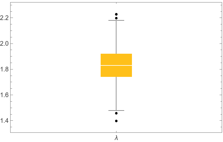
Bootstrap sampling is useful to get a sense of the range of possible models that can be fitted to the data. In a bootstrap sample, the original dataset is sampled with replacement (using
RandomChoice), so the bootstrap samples can be larger than the original dataset. No validation sets will be generated when using bootstrap sampling. The following sub-options are supported:
| "Runs" | 5 | number of bootstrap samples generated |
| "BootStrapSize" | Scaled[1] | number of elements to generate in each bootstrap sample; when specified as Scaled[f], a fraction f of the dataset will be used |
The "ValidationFunction" option can be used to specify a custom function that gets applied to the fit result and the validation data.
The
"ParallelQ" option can be used to parallelize the computation using
ParallelTable. Sub-options for
ParallelTable can be specified as
"ParallelQ"→{True,opts…}.
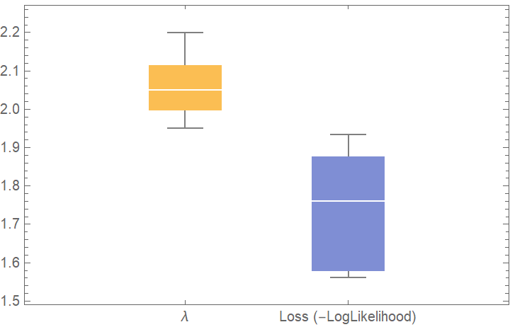
![BoxWhiskerChart[{{val[[All, "FittedModel", 1]], val[[All, "ValidationResult"]]}}, "Outliers", ChartLabels -> {"\[Lambda]", "Loss (-LogLikelihood)"}]](https://www.wolframcloud.com/obj/resourcesystem/images/27b/27b02800-4e9d-4ff6-8a0e-46bbb178d668/43b85962e31f3a1d.png)
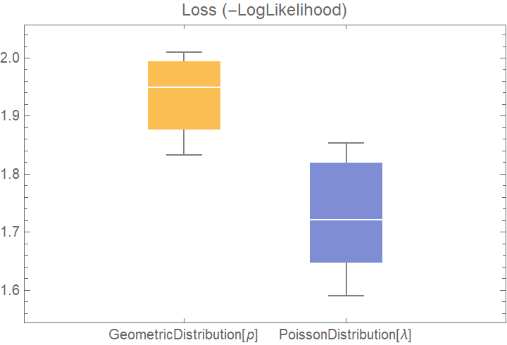
![dists = {GeometricDistribution[p], PoissonDistribution[\[Lambda]]};
val2 = ResourceFunction[
"CrossValidateModel", ResourceSystemBase -> "https://www.wolframcloud.com/obj/resourcesystem/api/1.0"][data, dists];
BoxWhiskerChart[{Merge[val2[[All, "ValidationResult"]], Identity]}, "Outliers", ChartLabels -> Automatic, PlotLabel -> "Loss (-LogLikelihood)"]](https://www.wolframcloud.com/obj/resourcesystem/images/27b/27b02800-4e9d-4ff6-8a0e-46bbb178d668/0685505abf3f4801.png)
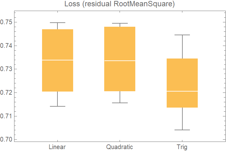
![data = Flatten[
Table[{x, y, Sin[x + y] + RandomVariate[NormalDistribution[0, 0.2]]}, {x, -5, 5, 0.2}, {y, -5, 5, 0.2}], 1];
crossVal = ResourceFunction[
"CrossValidateModel", ResourceSystemBase -> "https://www.wolframcloud.com/obj/resourcesystem/api/1.0"][
data,
<|
"Linear" -> Function[LinearModelFit[#, {x, y}, {x, y}]],
"Quadratic" -> Function[LinearModelFit[#, {x, y, x y, x^2, y^2}, {x, y}]],
"Trig" -> Function[LinearModelFit[#, {Sin[x], Cos[y]}, {x, y}]]
|>
];
BoxWhiskerChart[
Merge[crossVal[[All, "ValidationResult"]], Identity], "Outliers", ChartLabels -> Automatic, PlotLabel -> "Loss (residual RootMeanSquare)"]](https://www.wolframcloud.com/obj/resourcesystem/images/27b/27b02800-4e9d-4ff6-8a0e-46bbb178d668/5f96d32aeb273e70.png)
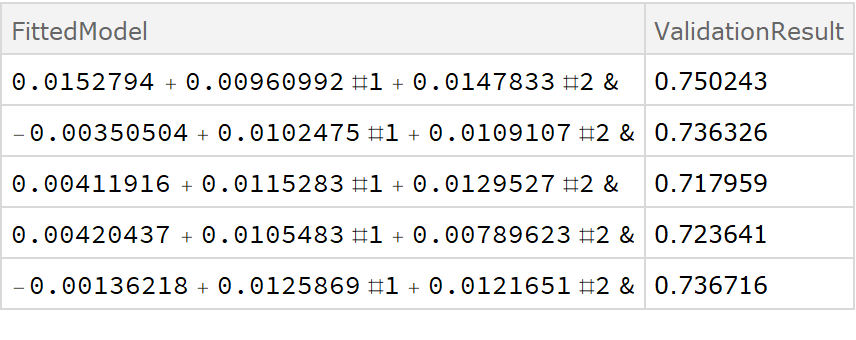
![crossVal = ResourceFunction[
"CrossValidateModel", ResourceSystemBase -> "https://www.wolframcloud.com/obj/resourcesystem/api/1.0"][
data,
Function[Fit[#, {1, x, y}, {x, y}, "Function"]]
];
Dataset[crossVal]](https://www.wolframcloud.com/obj/resourcesystem/images/27b/27b02800-4e9d-4ff6-8a0e-46bbb178d668/018d7a439521114f.png)
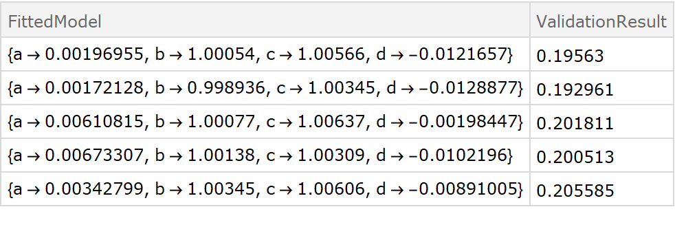
![fitExpression = a + Sin[d + b x + c y];
crossVal = ResourceFunction[
"CrossValidateModel", ResourceSystemBase -> "https://www.wolframcloud.com/obj/resourcesystem/api/1.0"][
data,
Function[FindFit[#, fitExpression, {a, b, c, d}, {x, y}]],
"ValidationFunction" -> {
Automatic,
{(* specify the fit expression and the ind*)
fitExpression,
{x, y}
}
}
];
Dataset[crossVal]](https://www.wolframcloud.com/obj/resourcesystem/images/27b/27b02800-4e9d-4ff6-8a0e-46bbb178d668/65c6604fac270555.png)
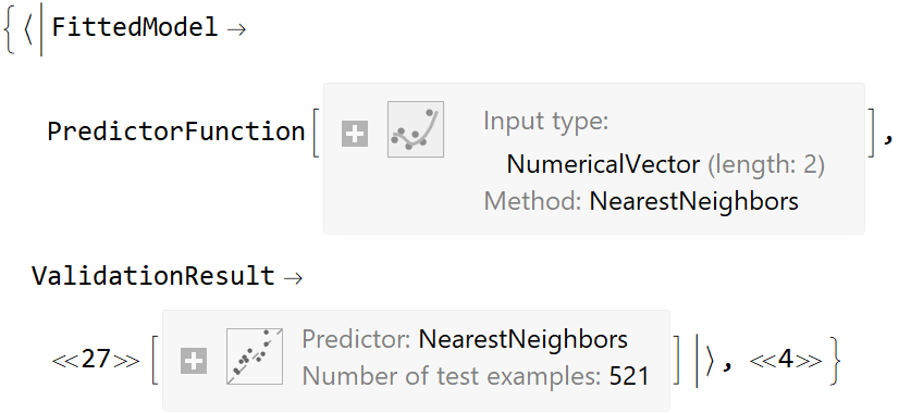
![data = Flatten[
Table[{x, y, Sin[x + y] + RandomVariate[NormalDistribution[0, 0.2]]}, {x, -5, 5, 0.2}, {y, -5, 5, 0.2}], 1];
ResourceFunction[
"CrossValidateModel", ResourceSystemBase -> "https://www.wolframcloud.com/obj/resourcesystem/api/1.0"][data[[All, {1, 2}]] -> data[[All, 3]], Function[Predict[#, TimeGoal -> 5]]] // Short](https://www.wolframcloud.com/obj/resourcesystem/images/27b/27b02800-4e9d-4ff6-8a0e-46bbb178d668/2d3d997a2c9f5a8f.png)
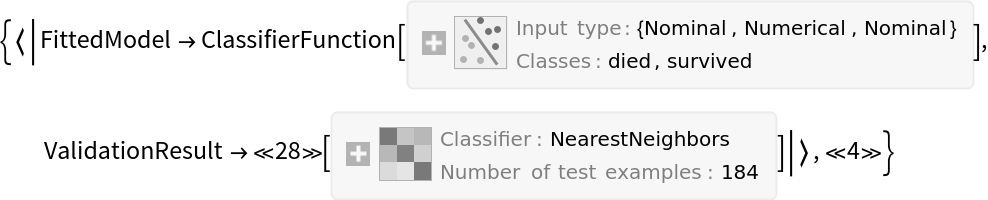
![ResourceFunction[
"CrossValidateModel", ResourceSystemBase -> "https://www.wolframcloud.com/obj/resourcesystem/api/1.0"][
ExampleData[{"MachineLearning", "Titanic"}, "TrainingData"], Function[Classify[#, TimeGoal -> 5]]] // Short](https://www.wolframcloud.com/obj/resourcesystem/images/27b/27b02800-4e9d-4ff6-8a0e-46bbb178d668/35a4572a90de4f33.png)
![tab = ToTabular[ExampleData[{"Dataset", "Titanic"}]];
ResourceFunction[
"CrossValidateModel", ResourceSystemBase -> "https://www.wolframcloud.com/obj/resourcesystem/api/1.0"][tab -> "survived", Function[Classify[#, TimeGoal -> 5]]] // Map[#ValidationResult["Accuracy"] &]](https://www.wolframcloud.com/obj/resourcesystem/images/27b/27b02800-4e9d-4ff6-8a0e-46bbb178d668/45d5265477338885.png)
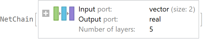
![data = Flatten[
Table[{x, y, Sin[x + y] + RandomVariate[NormalDistribution[0, 0.2]]}, {x, -5, 5, 0.2}, {y, -5, 5, 0.2}], 1];
net = NetTrain[NetChain[{10, Ramp, 10, Ramp, LinearLayer[]}], data[[All, {1, 2}]] -> data[[All, 3]], TimeGoal -> 5]](https://www.wolframcloud.com/obj/resourcesystem/images/27b/27b02800-4e9d-4ff6-8a0e-46bbb178d668/75793deef93af445.png)
![val = ResourceFunction[
"CrossValidateModel", ResourceSystemBase -> "https://www.wolframcloud.com/obj/resourcesystem/api/1.0"][data[[All, {1, 2}]] -> data[[All, 3]], Function[NetTrain[net, #, All, TimeGoal -> 5]]];
val[[All, "ValidationResult"]]](https://www.wolframcloud.com/obj/resourcesystem/images/27b/27b02800-4e9d-4ff6-8a0e-46bbb178d668/1ad6a612dde3c453.png)
![locs = GeoPosition[CompressedData["
1:eJxtWWtwldUVTYhF8RVUxjg0EStQwYhmBohSKXMtyWg7UdIoIxVytYLU1BrJ
m0tCNPcmuY8MJWInxRFQ8YHxWR0JaoseoSptWkVw0kZjldSWIS2DpZDJmLZ6
1v6+mbP2sb+Sb77H2Weftddae99v3X5PxR0TsrKyTmRnZeHvmyt+e/rSxtKI
/dc81BE1a4uP7tvQFFyftNcXXjk+nGqV68jOeNT07I82TV8fXL/fHjXVK3av
/1NtcP1CKmrSuafd3V8TXM/siprrn07OXxG8b3o7o+bz98orZzW654vyx25c
sCa4/1kyaloKpqSuaHXXqZxvP7JsXfD8jraoWdJXNeG9huD+iL3+Rvcmc2oY
75PpqDn7p3vOeL05eH7YxnvF5POTb68N7l9s159dcNb4i+H3FtjryY2P/7mo
Lrg/J6P302T3t6rxmTueD/Oz2cb7YqJ3dV5LcP9op1rPHLTrf9F731N/Wefi
O9HXlP/74Hlzi/3+zOK/Xz25Pni/xF6fX/XcqtIgX6YiETUH5n/y/KY1Ll8U
f+TMTp0P5H9KZf8vD8SC65Tdb/2Styf9M3g/8riOX95f1v3g9R1hfPfa9bK2
puf9O8zPyjZ1Lef9Yc6cOQPr3X5v3dj+5Jnh99fZ599Z8seeqnq3v6qql/+1
p949z3ipT+p4xu31nZUHZpQH982dXXq9vTa+m3prf/7XOoenixZ//MJ4cP6R
vIzaj8Sz6ciVr7SF5xWz57Fl709yrmp25/fslviOhhA/Uyy+s3vvyl4d7qfD
Xp+eeKgsv8Gdz9TyD6YfDvAV2ZZR+xE8Ub1Euu16fzuyqPTLmKsf3t9bKY3/
Mfu9zUORkp56l4++xpeOF65z+eT94TwIT5Fiu54pH/7ucKuLl/BrJtrzf6b7
kQ8nhPU0YOMdys394roGFy/fn5ZW9Sj1MS9n2nkfhfmssetvGL38srtDvGRs
vH/43sDFrWG9ZNv70cT2wQfD+2VpjY+ru3S8/Rldj8j/QP7E6nlNDj983uAL
rqeSuKoHk8yo9aR+Kd5IQbvKb2RZh853nv1e2+SCKSVhfj+weDq2t7p7Zxjv
7rSqX9PSqflialLvH3jj+i20640MXfv+eWvd9+j8pf75fHrs9W+qft0aWev4
5K3F//jdaIvD18/KP/rVqhDfgwl9fqgXil/y9Z+dtzf8sNbla9HHN0Tvb3Z8
Qfxt9tnvvxL/xRvbahx/fDo6/9WRZldfO3pj3/xxyL9nd+n8jaQ13n/QrvkY
eCrZf/PIEzG3HuO9yu6ndGjBrgtqHH/cuLX7zTUtjh/4++B71g/wGfGx4Kd1
9uhN28P6L0qq68hSj9+x/mN7Kla8EfJxZVLz41BK5SNSk1H1YLrt+v3FJ5ae
0ezwwfzyeULzIeqxcPaxd2aEeDKdGs/gH9Y76A3zK/DEeg5+Z367Nqn1ZRH2
u7FrbqbO1TvX3w7Np1KvjLeXMxrf4F+KX/DA5wW+Yj7HNfMJ9I7zVWHfT+R/
+Wlf+Hw8pfXlXbufq0ZKD7SE/DrX4uuWLc1Tx2ocH7EfWObVH/DJ9QV+pPyI
vjD/od6mX3rKPVvD/bzUofBudrcpvAh/cX3P1Xxk+uP6/oZ2zW+77P6+M3rJ
w8fC+1kev6EeWV+eTej3Bzz8oH6IX8RffX/vbY2vNTl9mtT06r296x1fMp8B
/6Sfwi/MB4if9w/+Zb4BHzKfXK7rX/DA51ndoesf9bC9b83GspjTT8YT9IPr
FfrM65Xo+hF8sf5Br9g/wI8wn3r5Fn3gej/crvVsuefHsD/SM8nH4ZMXnVtb
83/zb15rV/458kCn5g/4gciRosJT6pwe0X7Fz+6f/d9D02KO36m+RL9Z34AP
9sOIj/GD9ZlPV3cq/pf6Yr3v1/os/Mf+blJa4xV8xHyB9divoR7o/IVfmQ+h
H4zfWTp+2Q/nE/zNeoX9UHxmpq2nQxMu6Kysc/HReZocrR+Sb+6fUI/MD8BT
7eLPFsZi7j7XE/iX9RrnT3wl9cr+E+8zn6E+OB7kh+MHPljfwO/Eb1/TU9xn
PwJ+p/ORfpHPB3rK5wk/yf0j6o/9V4X2g/I+6ZXZFtf+b5bnn1emNd/M8vzh
oJd/4IP4XvSQ+EPyNbrnR0cWhniHn2C+We71Q/AH3O/BDxFfSzzkR0SP6Dxk
fT5v4I3PB/pD+ZN88vrwD4znmZqvhM/YH6A/5PjAz+wXwN/Md7s9vlri9bu3
tWv9wH3iG/EnrF/wn4wnxMv9J86f/VSe7rcEn4xX6C/rJ/wI8aHwC/tT9EPk
J0TPma/9/gJ6x9+Hn2G/CP9BfkTOj7+H/pz8lDme0v1CbkL17+ZQRuenUPej
Ej/3K9A3zi/6F/bPOD/Cs+yX+9ls3c+JnnD/Cn7h+kP9Ml7hLwg/wv/s78EP
7DdRz+SfxP+TPxB/yfGj/+H+xJ/HoH9hvSvS/lrywfUOvLE/9fy8+A2OF/zL
/SXqm/hb/CN/77Cex5hzUto/e/Mw8SuML+SD9XqbN4866p03/CbrIfSW9QD+
jfyUnDf3GwsTWu9LPH7o9vgj16s/+AXOL86H+Rt45edRDzS/k/pkvkC/wvX7
rvabMg9hv4j9sR9CPNw/fdKh6xV8znpzTYeeX/R7fvJR7TeE79kPQX9ofifn
w/oB/LL/qffmXfDzPA+BXjB+x+Ian4Nan6W+uH8G/ng+l6vnB8KX7IeyvPlW
3OMn4IP91S5PL8s8foG/4Pkv6oPnv/BL7Od3ev6w2JvXgQ+5XoAH9p9NGk/C
z+zfD+r+TvDM+RzQ/lXqj/kb+WO8xj3/8T+vvgo03/vzJuEXnk/kef3pJG9+
uEjPF8xdHj6Qf65f7If0WPw2nzf4n+c7g57+oP7Yz8PvsB9HPfG8AP0X85s/
/wJemC99fAHv7B9QjzzfxPnyvBr75fhX6v5LzpfjwzyV/SfqkeYX0l9wPwe8
Ml8N6/5N/CPjDXrD64EPmP/gJ1lfezz+gJ/meQL4mfpRf94m/MF8mNF+W/SC
6kv0jfth+COuB/AV6yvmX6x313jz2GIvv6hf1kvoEdcH4mG/Cz7leRH8AuFF
9JD58wH9+4H4B/Zb+zw+q/bmoSc9/1TpzVPgx1h/MJ/h/MFvc3+I+Jmfxrzf
l8C/rDd4nv0m/DXzJfp97oeAD/bj4Ge+PujxI+bpPF/B71/sr6DnHA/6XeYX
5I/5Y6Kn3wN6HiffJ7x8LT/wz+x3Ma9mvkf983roH/j3MOCP9bfE+30A+Od8
lHn9FvDJ+IV/5XkS+I71EfhlfvfmraI/rDfLvd9fEB9/D+9zv4b64fPyfq8Q
/uP5C95nP4H+mPfv1ZPMS5mfsz3/j3yxHoKPaT4q+sLzCHyP/cC41lupD56H
Ar/cr2B92q/UM/dTx715l9d/ST1xfcN/M1+jH+LzhZ8gPEv+WH+Qb/Yj6B/Z
b8PPc38OvWf+Qf4Z/3P073XCd18BK2fXbg==
"]];
vals = CompressedData["
1:eJwVV3k8Vt8TRvY9IooKoSiRQioGZUtEpRBlKRUpW4mkleSnb0gL73vvua9S
VCoilLJFe6KUrSJboizJEvrN/eedz5w75565Z2ae53nVfPa77OTn4+P7jT/O
wY1TIMeFe/efjpmjvVqzw6rEkgPpV62+xQxyQWHdDrumKxT8nWtOJZ3mgEKZ
quqWozTcf7VAqX86Fxpz85I+F9Hwc80Lv1meBHRPytHFPhToqW68a7+HBw1X
709rwrhLoimtmY/xPdG3F1nhOfLq2U8c0G6f1NbJX0zDi7xbT9RbCehDe+Yw
xk8pfLtric8FnbRTR0cJPN59V7gwjYaoFX+Hh/QJnLTdP79QDfOwfz178wsK
XN165PnkCUQvGw1ci/vOdcodCGLPOeKxznk/AbdVox8M/9Bw56avvgmu68o4
y5xHO5m/Pcmji0CdxICjQzgDKTJd0VobCWjmx5qE89LhoWf3xwcfaFDbNhah
gPEJQh8LTAcp6NbtmyGM/sdTc5Vf9VGQkZHyhkqmYLWsTyKlTIMt3yXybCHm
L6ra/ESYApfwyOJm/C43LeEoWdy33HrBVlu0JtsyT0u5EfDqfWDx5X8EKhX4
lJ5eo0BjKrLWM5OGugm++K/KXLBu7l7jhPF8O1OrJLIYaLd0PflpDQH++K1T
o60UZNUEFfY2E7ARH4xzViVw/ky/jmA8A1t+FnWOyxIwlA0e1nYmwLxYr7dg
IYFTE479tfwUcOwOvxVNISAd8YiIZnPht4S0va0qD5zWNvqp4HmG2j7lUSe4
QN6v+92nSsErxUWm9GYa+qs0DneuoIGKsfrkhXGOJW5/56NNPBUp/Au/k8vr
i3pkxoWtc5Tze2R58MOd33qDNA2cufaHQzGu5OOk1A60NyZsVt2pp2FEoT2g
4g0F2fsvCQruxfuuXzebPd/Ivc1IYIABo6On9PjR//1E8LYHu6/IquSzMxfm
n+WsNfIlEGnkmrLcggE9Jz/NjUkMXHDw2e69lAvg81gpcRYFzouvpMQ95cLG
iECZ53/S4dJVOYHM21zo2Od5NhLfJyml5DEnm4bxRqMsxVk0PG9vEpryY+As
n8CbxjMExNRnvRy9QWBg5KA5m7fq7Ec1jk8I9J4KSHdGn5eRpZ/M5muk3zay
iYBHmtFQaiYFvgb9r2A9A/0hjv81lmM/mVdISWKcy1Sp1Qz2O5pj1v7B++r9
dc6d00PDTB++dyOLCKjv/iQzgevGgglO/Xh+R1Fq1GkfLiQfKn1hjPtEk5Nr
9LkMnMjp8GDnK1ZpyFXQjgFpTtCJu1if9OnXtOtx/W7/9rzJ89jfX9N1Tb0Z
SEobjfiF/Sxhc6zxYzQFbllLMmTwO1Q8NRNcmhiY4KsXbE4jcGURo/jjGYHL
L26OuC1kwJA7c83FaxywPmahP62FAd2znN7vhdhX9/bsMcR8DPaZrm7NIcAJ
l43vwPdvkqvOnxrG/jbufGO7ksAXZ+OBQwJcqDkuWLMH43PPmTQ0YH5lrfWV
i9FfncndUydNYGvAvriV6D+QMFLdhXbEQv3I01oK9ibK7phchuftbPqmu4LA
7FvfT9nhHNz50evq5EODqozY/wwwXspDbEdbEIGXVflhC9E3y06+xcX5S5Y3
1bHr4cIa9U6eUCQXUrxuFPzD8++kXjQeQTvtyf5w+yUExmgXZXXcd39Z2sD1
SRoq5rr3H1XkgteFw6VGrjQEL3c0aXSjIH3escjgHA40x304xNbvkwBn7goJ
An0V0s/4SgiIr30f09rLwGVT/njlhwxc81wTJt1IwXcPs9obA1zIOZAhVm9N
4BHPebOwEwG5wCcJmfk0zB94NiS5C3HiuYLPi2QO3C7UsFbpYuD0vv61rrMJ
ZA7tLyudToGi1w6fATZvJ4mWtw1cOERF5FgaE3iYWhnuFkmDsMlzE/NJAvar
clPF/xL4lHBixc31FDzQshcPwO87IjQutwhtUUdup9oQgcObZzR/aUAc69LT
ZefuWtLIKju0/t8ubXVEu+tDYNXKeAIF1sUctt7Wfer/iTUREIh9mDL9PwJl
711nsHGWs78HCqGtOJ5xKn+KhkkRTQUL9FflqNgoFBH4ti3o7RBBPJYfjpKy
IGA0a142Oz8ORxSFcn5yoKNZWm34MoENdGPLhAmB8JA2yTZLAm3vx10jsA66
GqInq8JpiJHQ+HsK940e7fiqi/ZfpPu7hAIauAEpAyy+3tMoPs+ZQ0GZScSo
Hvp2K41EHZdkgPdl0ycSBgwUiE1tryqm4OQ33guTdQTqWw5+czzNgwtbJKrX
+/PgXOJzF3/cp5Awqi2P9nrVn51CHxgQ+fT7x1AWDeI6no2fpXlQN1wyoRlD
wHbC9aYX8ibnsN/sSaxL2lS/aAvadvMppyYFxEuxxVOp9Xj/4ZUF3vi+1C5V
W7bPHheZUv/V0pCbqaxtakMglfmc5hxNoOSCVtx1ccwb1DTY/tLXKExi7cII
7ZGXP9PhDey/y2/MA4fPBWl5uziw+X3P2+FMAo3ONbEzOmlIHNAOSMulYV7I
0Z0Nrykw2CVeXTSGfVd6NKyQxwWnVW01GzHu7uqj01g81WyjhXIYLkQuiRNh
5zGnTcTsBNp2eaLK8mV//SL3Njx/W9hAhhXWXUzoZVjdLOT7WXGNC/D5tlCX
TcOPCPBJavum4byquO1fxPK3TpGOyh2GhuyJLIk6Lg2Dqm+LWF5+8FdLSDuE
hu4f1yUk0C/2fCTJzr3HIz+qVouAdu0yY0H0Q+x4vSYBBGTeV2UcQL9O38SJ
5RctQ/u9u0K4cOsWY9JezoPlSZtFWN733Hy8ckkKAwFy09+tY/Hj3zre2g7E
6crAql7cV9/SHKOD6/YDA/0baAaUynwS7X0ZyJP643sG19/F3i6pQF3hfbEt
ZJMlDfc+XTlvg+tq8QacDSwu7D45vN2aA0EHrTUeFHOhaXD/faqPA98nynsT
8XnWxf6Bo2j7dnofKV1OQ8Co3rTJ+wT0gq6YW48QCH30SrR5DQP+fA9jJ1QY
CL8TrO2K8ZeN/lguQX1S58YsGMI8Cz6KtreydS90lp2dwUBDRfFtRYwLvqQq
9nEp9sexBotwdRqiszP2wFMCUa/ahDsvEPjYmxgqKM+DCgPOJTvkg7yPWfsd
PhAIE2rRD8b95rX3PKuxT8NWaBwyw3u6467VEdmI+HVW0b/7IIFsC+ecm8j3
0swPGVbv3FLY9JjFa/GkZQlmWFcyViqwFf2WpxKR7ZifUklEf+xSGlYrmJWM
FTKgnH9E4QvOd6pDiH8Uy4uhesrirI64Xn1xDvK8aXY4n7kYA5IbHG1jcij4
tm/ZK3qSAzuaHBqn2gnOqa3hWR4F/5SW6H3PRpwffqvzj0Mg/r3YsG85DU2K
l23Y+hkc0tk3vgrXB7sfKyUR2P2SXrQK8cXKZs76aHy+1aurmdWz/EXx79g5
DuVbbOASywEbk8Uz2L7gl/le9XUegWrX9J0sD6RX23r5FHChe/jnMhm2z4ql
S7orCdxDrFVFP3CDV1zeJAU3TCtz1l+kYavG/ffeJziwYfnq6HF2Lt8umtE9
SODZhV9KKg8J9D+XOMPqilq522b1AohjVeWSdRg3XnKPaUc9bX2sQnYpPtcS
zplhv5AHfRN+XesVCNyPfJQ1iHHTayxUWL0X9MH8u50mgcXbMkJY3Nb+srDO
k9WPk1ebn/ekw420sc0is7BeeSrDcrieHl/poszed2qlVIMBBfO6gouES3hQ
5vE6S4PVJ3scrrN4Wf1g0yYtA+Sdi+tOJqDfoC2vvE4b++bElaOsvlm5tNqT
8aTg1uMhSZYPvv4cea6EVtZQpkiU5dWfcRd/qzMw7c3bZy7oz9Yoc7RC/Mqz
Pi05hvlHRXfrnxKnoPeyY8VXxG+B4GLNsYM8SHbZfeU6zs2ZwYzX7FwFla/I
+WtPIL2zW8/KiQex+f/WK52gYfG1Bi+2/+avvhXWifU3PXZwMLwxHQyM9pke
wzrNaRHMtjdm4Ny105fL8PtvF27y2HmWBpvP5cksPy2POSPE9l3Isl06/eIE
9nar8I95ob7Wz1K7dBjv5YxaFHsPNyeWF7L3pTC2Y7sv2t31dnO7Mf9DPZYB
oa4UTCr4BIaOp4ORrndEyxsCKRk92pOiPJgWEW+1hcXHXw+LWf5q+C0nMhtt
98sw1wL8PufX/lvY+kqnBnipYF3Dnkt+YuPju8K9Wf2XKvEgshX1q7rPpZZw
th9jpc0rEZ+ztxW16qOvqHRtK5NMw0HbOZY+6L+VNatj713jVoK/XRvqkD9V
Pf2oc/JC791g6xcmMUfzNeZdND9YoJbVVSXlk20FBDJGvQS/oK4au1K1+SHq
cZjnq81+30Tts6qNLF6NPHNzCcL/b0Wx/xsvoSGO2mM4iHnox+Z1TmN509NP
RDyUgDthEpxkeKC+8sCR9x8Q74kxv+ZxAjPlNZf9wb6/s+Xd9AcdOLfJnh6s
rthc1nnkK57j0F+5rRH/J2jJFV8/i+uDYeF70mJRFx9/rOK+lAM9fYO583C9
NLtKLQt5/bbwoUZXMQL/tmebDJsRuCtv7jJuQcP0zB8Lo7VoOPO6SzkXeV5P
4bzvTFY/1028cTVDHhEBv3gpxNEQvcAeigGbBf5xYtUMrI5xOFAai+eW5Duz
9c6dMBll+SbRP1SntYGGVx8Umlag/6p4bYIU28fuN+WPo13onTHK6qsdu7ya
bBBHb2RdVmDr8FPcrFFkPQ/u/HYhM01ZHbBp2FED533tTysH5LP8y95qgRjn
Z873aznaBa45paZsfQxlrTfg/6+dwinu2qgTQ2fWxHaXI18n++/NzeTAUz6n
e+moE6JXjV0fCGKAypRwtxVh4P8qoCo5
"];
SpatialEstimate[locs -> vals]](https://www.wolframcloud.com/obj/resourcesystem/images/27b/27b02800-4e9d-4ff6-8a0e-46bbb178d668/112862ac353e26b0.png)

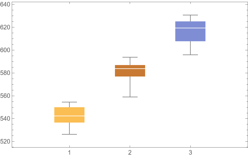
![unpackedLocs = Thread[locs];
result = ResourceFunction[
"CrossValidateModel", ResourceSystemBase -> "https://www.wolframcloud.com/obj/resourcesystem/api/1.0"][unpackedLocs -> vals,
AssociationMap[
Function[degree, SpatialEstimate[#, SpatialTrendFunction -> degree] &],
{1, 2, 3}
],
"ParallelQ" -> True
];
BoxWhiskerChart[{Merge[Identity]@Lookup[result, "ValidationResult"]}, ChartLabels -> Automatic]](https://www.wolframcloud.com/obj/resourcesystem/images/27b/27b02800-4e9d-4ff6-8a0e-46bbb178d668/018cc0496ec18d2e.png)
![crossVal = ResourceFunction[
"CrossValidateModel", ResourceSystemBase -> "https://www.wolframcloud.com/obj/resourcesystem/api/1.0"][RandomVariate[PoissonDistribution[2], 100], PoissonDistribution[\[Lambda]],
Method -> {"KFold", "Folds" -> 10, "Runs" -> 4}
];
Length[crossVal]](https://www.wolframcloud.com/obj/resourcesystem/images/27b/27b02800-4e9d-4ff6-8a0e-46bbb178d668/04a845a788cfa70c.png)
![crossVal = ResourceFunction[
"CrossValidateModel", ResourceSystemBase -> "https://www.wolframcloud.com/obj/resourcesystem/api/1.0"][RandomVariate[PoissonDistribution[2], 100], PoissonDistribution[\[Lambda]],
Method -> "LeaveOneOut",
"ParallelQ" -> True
];
Length[crossVal]](https://www.wolframcloud.com/obj/resourcesystem/images/27b/27b02800-4e9d-4ff6-8a0e-46bbb178d668/6996e7449270b070.png)
![ResourceFunction[
"CrossValidateModel", ResourceSystemBase -> "https://www.wolframcloud.com/obj/resourcesystem/api/1.0"][RandomVariate[PoissonDistribution[2], 100], PoissonDistribution[\[Lambda]],
Method -> {"RandomSubSampling",
"Runs" -> 100,
ValidationSet -> Scaled[0.1]
},
"ParallelQ" -> True
] // Lookup["ValidationResult"] // Around](https://www.wolframcloud.com/obj/resourcesystem/images/27b/27b02800-4e9d-4ff6-8a0e-46bbb178d668/5020fb61651b9dcf.png)
![ResourceFunction[
"CrossValidateModel", ResourceSystemBase -> "https://www.wolframcloud.com/obj/resourcesystem/api/1.0"][RandomVariate[PoissonDistribution[2], 100], PoissonDistribution[\[Lambda]],
Method -> {"RandomSubSampling",
"Runs" -> 100,
ValidationSet -> Scaled[0.1], (* This illustrates how the default "SamplingFunction" can be replicated as an explicit Function *)
"SamplingFunction" -> Function[{nData, nVal},(* The sampling function accepts the number of data points and number of validation points as inputs*)
AssociationThread[(*The output should be an Association with 2 lists of indices 1 \[LessEqual] i \[LessEqual] nData *)
{"TrainingSet", "ValidationSet"},
TakeDrop[RandomSample[Range[nData]], nData - nVal]
]
]
},
"ParallelQ" -> True
] // Lookup["ValidationResult"] // Around](https://www.wolframcloud.com/obj/resourcesystem/images/27b/27b02800-4e9d-4ff6-8a0e-46bbb178d668/2131f040e9e401f4.png)
![bootStrap = ResourceFunction[
"CrossValidateModel", ResourceSystemBase -> "https://www.wolframcloud.com/obj/resourcesystem/api/1.0"][RandomVariate[PoissonDistribution[2], 100], PoissonDistribution[\[Lambda]],
Method -> {"BootStrap", "Runs" -> 1000, "BootStrapSize" -> Scaled[1]},
"ParallelQ" -> True
];
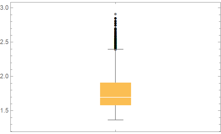
BoxWhiskerChart[bootStrap[[All, "FittedModel", 1]], "Outliers", ChartLabels -> {"\[Lambda]"}]](https://www.wolframcloud.com/obj/resourcesystem/images/27b/27b02800-4e9d-4ff6-8a0e-46bbb178d668/7abde33aefbe7bf8.png)
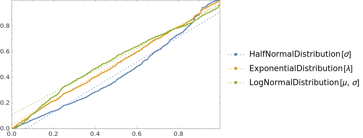
![cdfValues = ResourceFunction[
"CrossValidateModel", ResourceSystemBase -> "https://www.wolframcloud.com/obj/resourcesystem/api/1.0"][
RandomVariate[ExponentialDistribution[1], 1000],
{HalfNormalDistribution[\[Sigma]], ExponentialDistribution[\[Lambda]], LogNormalDistribution[\[Mu], \[Sigma]]},
"ValidationFunction" -> Function[{fittedDistribution, validationData},
CDF[fittedDistribution, validationData] (*This should be uniformly distributed if the fit is good *)
]
];
QuantilePlot[Merge[cdfValues[[All, "ValidationResult"]], Flatten], UniformDistribution[], PlotLegends -> Keys[cdfValues[[1, 1]]]]](https://www.wolframcloud.com/obj/resourcesystem/images/27b/27b02800-4e9d-4ff6-8a0e-46bbb178d668/5e6807ccf5c72854.png)
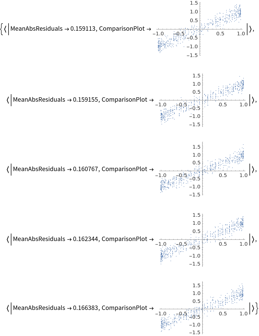
![data = Flatten[
Table[{x, y, Sin[x + y] + RandomVariate[NormalDistribution[0, 0.2]]}, {x, -5, 5, 0.2}, {y, -5, 5, 0.2}], 1];
ResourceFunction[
"CrossValidateModel", ResourceSystemBase -> "https://www.wolframcloud.com/obj/resourcesystem/api/1.0"][
data,
Function[
NonlinearModelFit[#, amp*Sin[a x + b y + c] + d, {amp, a, b, c, d}, {x, y}]],
"ValidationFunction" -> {Automatic,
Function[{fittedVals, trueVals}, <|
"MeanAbsResiduals" -> Mean[Abs[fittedVals - trueVals]],
"ComparisonPlot" -> ListPlot[SortBy[First]@Transpose[{fittedVals, trueVals}]]
|>
]
}
][[All, "ValidationResult"]]](https://www.wolframcloud.com/obj/resourcesystem/images/27b/27b02800-4e9d-4ff6-8a0e-46bbb178d668/14755d9e6bd401df.png)
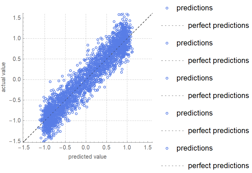
![data = Flatten[
Table[{x, y, Sin[x + y] + RandomVariate[NormalDistribution[0, 0.2]]}, {x, -5, 5, 0.2}, {y, -5, 5, 0.2}], 1];
ResourceFunction[
"CrossValidateModel", ResourceSystemBase -> "https://www.wolframcloud.com/obj/resourcesystem/api/1.0"][
data[[All, {1, 2}]] -> data[[All, 3]],
Function[Predict[#, TimeGoal -> 5]],
"ValidationFunction" -> {Automatic, "ComparisonPlot"}
][[All, "ValidationResult"]] // Show](https://www.wolframcloud.com/obj/resourcesystem/images/27b/27b02800-4e9d-4ff6-8a0e-46bbb178d668/7f82533ddfe1da52.png)
![data = Flatten[
Table[{x, y, Sin[x + y] + RandomVariate[NormalDistribution[0, 0.2]]}, {x, -5, 5, 0.2}, {y, -5, 5, 0.2}], 1];
net = NetTrain[NetChain[{10, Ramp, 10, Ramp, LinearLayer[]}], data[[All, {1, 2}]] -> data[[All, 3]], TimeGoal -> 5];
ResourceFunction[
"CrossValidateModel", ResourceSystemBase -> "https://www.wolframcloud.com/obj/resourcesystem/api/1.0"][data[[All, {1, 2}]] -> data[[All, 3]], Function[NetTrain[net, #, All, TimeGoal -> 5]],
"ValidationFunction" -> {Automatic, "MeanDeviation"}
][[All, "ValidationResult"]]](https://www.wolframcloud.com/obj/resourcesystem/images/27b/27b02800-4e9d-4ff6-8a0e-46bbb178d668/681d948930f65259.png)
![(* Evaluate this cell to get the example input *) CloudGet["https://www.wolframcloud.com/obj/b4bbb588-a49c-4389-9e7a-c129fc7bc94b"]](https://www.wolframcloud.com/obj/resourcesystem/images/27b/27b02800-4e9d-4ff6-8a0e-46bbb178d668/20a0ef46d8187e81.png)

![ResourceFunction[
"CrossValidateModel", ResourceSystemBase -> "https://www.wolframcloud.com/obj/resourcesystem/api/1.0"][RandomVariate[PoissonDistribution[2], 100], PoissonDistribution[\[Lambda]], "ValidationFunction" -> None]](https://www.wolframcloud.com/obj/resourcesystem/images/27b/27b02800-4e9d-4ff6-8a0e-46bbb178d668/77221a864dd9a031.png)

![crossVal = ResourceFunction[
"CrossValidateModel", ResourceSystemBase -> "https://www.wolframcloud.com/obj/resourcesystem/api/1.0"][RandomVariate[PoissonDistribution[2], 100], PoissonDistribution[\[Lambda]],
Method -> {"KFold", "Folds" -> 10, "Runs" -> 500},
"ParallelQ" -> {True, Method -> "CoarsestGrained"}
];
BoxWhiskerChart[crossVal[[All, "ValidationResult"]], "Outliers"]](https://www.wolframcloud.com/obj/resourcesystem/images/27b/27b02800-4e9d-4ff6-8a0e-46bbb178d668/07f0099927bc32e5.png)
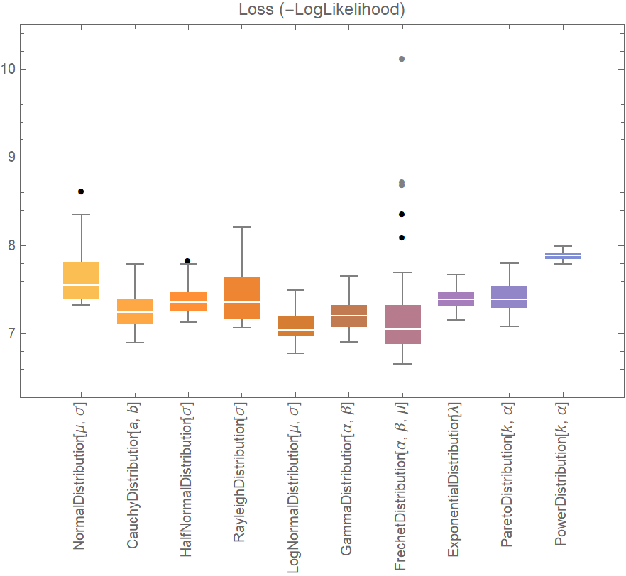
![data = ExampleData[{"Statistics", "RiverLengths"}];
dists = {
NormalDistribution[\[Mu], \[Sigma]], CauchyDistribution[a, b], HalfNormalDistribution[\[Sigma]],
RayleighDistribution[\[Sigma]], LogNormalDistribution[\[Mu], \[Sigma]],
GammaDistribution[\[Alpha], \[Beta]], FrechetDistribution[\[Alpha], \[Beta], \[Mu]], ExponentialDistribution[\[Lambda]], ParetoDistribution[k, \[Alpha]], PowerDistribution[k, \[Alpha]]
};
val = ResourceFunction[
"CrossValidateModel", ResourceSystemBase -> "https://www.wolframcloud.com/obj/resourcesystem/api/1.0"][data, dists,
Method -> {"KFold", "Runs" -> 10},
"ParallelQ" -> True
];
BoxWhiskerChart[{Merge[val[[All, "ValidationResult"]], Identity]}, "Outliers", ChartLabels -> Thread@Rotate[dists, 90 Degree], PlotLabel -> "Loss (-LogLikelihood)"]](https://www.wolframcloud.com/obj/resourcesystem/images/27b/27b02800-4e9d-4ff6-8a0e-46bbb178d668/4cfaf3d2b86375f7.png)
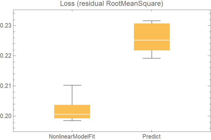
![data = Flatten[
Table[{x, y} -> Sin[x + y] + RandomVariate[NormalDistribution[0, 0.2]], {x, -5, 5, 0.2}, {y, -5, 5, 0.2}], 1];
crossVal = ResourceFunction[
"CrossValidateModel", ResourceSystemBase -> "https://www.wolframcloud.com/obj/resourcesystem/api/1.0"][
data,
<|
"NonlinearModelFit" -> Function[
NonlinearModelFit[Append @@@ #, Sin[a x + b y + c], {a, b, c}, {x, y}]],
"Predict" -> Function[Predict[#]]
|>
,
"ValidationFunction" -> <|
(* the default validation function will be used for NonlinearModelFit, so it does not need to be specified *)
"Predict" -> {Automatic, "StandardDeviation"}
|>,
"ParallelQ" -> True
];
BoxWhiskerChart[
Merge[crossVal[[All, "ValidationResult"]], Identity], "Outliers", ChartLabels -> Automatic, PlotLabel -> "Loss (residual RootMeanSquare)"]](https://www.wolframcloud.com/obj/resourcesystem/images/27b/27b02800-4e9d-4ff6-8a0e-46bbb178d668/70d3de0c677d7c86.png)