Details and Options
The recognized formats for
data are listed in the left-hand column below. The right-hand column shows examples of symbols that take the same data format. Note that
Dataset is currently not supported.
ResourceFunction["CrossValidateModel"] divides the data repeatedly into randomly chosen training and validation sets. Each time, fitfun is applied to the training set. The returned model is then validated against the validation set. The returned result is of the form {<|"FittedModel"→ model1, "ValidationResult" → result1|>, …}.
For any distribution that satisfies
DistributionParameterQ, the syntax for fitting distributions is the same as for
EstimatedDistribution, which is the function that is being used internally to fit the data. The returned values of
EstimatedDistribution are found under the
"FittedModel" keys of the output. The
"ValidationResult" lists the average negative
LogLikelihood on the validation set, which is the default loss function for distribution fits.
If the user does not specify a validation function explicitly using the "ValidationFunction" option, ResourceFunction["CrossValidateModel"] tries to automatically apply a sensible validation loss metric for results returned by fitfun (see the next table). If no usable validation method is found, the validation set itself will be returned so that the user can perform their own validation afterward.
The following table lists the types of models that are recognized, the functions that produce such models and the default loss function applied to that type of model:
An explicit validation function can be provided with the
"ValidationFunction" option. This function takes the fit result as a first argument and a validation set as a second argument. If multiple models are specified as an
Association in the second argument of
ResourceFunction["CrossValidateModel"], different validation functions for each model can be specified by passing an
Association to the
"ValidationFunction" option.
The
Method option can be used to configure how the training and validation sets are generated. The following types of sampling are supported:
| "KFold" (default) | splits the dataset into k subsets (default: k=5) and trains the model k times, using each partition as validation set once |
| "LeaveOneOut" | fit the data as many times as there are elements in the dataset, using each element for validation once |
| "RandomSubSampling" | split the dataset randomly into training and validation sets (default: 80% / 20%) repeatedly (default: five times) or define a custom sampling function |
| "BootStrap" | use bootstrap samples (generated with RandomChoice) to fit the model repeatedly without validation |
The default
Method setting uses
k-fold validation with five folds. This means that the dataset is randomly split into five partitions, where each is used as the validation set once. This means that the data gets trained five times on 4/5 of the dataset and then tested on the remaining 1/5. The
"KFold" method has two sub-options:
| "Folds" | 5 | number of partitions in which to split the dataset |
| "Runs" | 1 | number of times to perform k-fold validation (each time with a new random partitioning of the data) |
The
"LeaveOneOut" method, also known as the jackknife method, is essentially
k-fold validation where the number of folds is equal to the number of data points. Since it can be quite computationally expensive, it is usually a good idea to use parallelization with this method. It does have the
"Runs" sub-option like the
"KFold" method, but for deterministic fitting procedures like
EstimatedDistribution and
LinearModelFit, there is no value in performing more than one run since each run will yield the exact same results (up to a random permutation).
The method "RandomSubSampling" splits the dataset into training/validation sets randomly and has the following sub-options:
| "Runs" | 1 | number of times to resample the data into training/validation sets |
| ValidationSet | Scaled[1/5] | number of samples to use for validation. When specified as Scaled[f], a fraction f of the dataset will be used for validation |
| "SamplingFunction" | Automatic | function that specifies how to sub-sample the data |
For the option
"SamplingFunction", the function
fun[nData,nVal] should return an
Association with the keys "TrainingSet" and "ValidationSet". Each key should contain a list of integers that indicate the indices in the dataset.
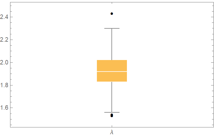
Bootstrap sampling is useful to get a sense of the range of possible models that can be fitted to the data. In a bootstrap sample, the original dataset is sampled with replacement (using
RandomChoice), so the bootstrap samples can be larger than the original dataset. No validation sets will be generated when using bootstrap sampling. The following sub-options are supported:
| "Runs" | 5 | number of bootstrap samples generated |
| "BootStrapSize" | Scaled[1] | number of elements to generate in each bootstrap sample; when specified as Scaled[f], a fraction f of the dataset will be used |
The "ValidationFunction" option can be used to specify a custom function that gets applied to the fit result and the validation data.
The
"ParallelQ" option can be used to parallelize the computation using
ParallelTable. Sub-options for
ParallelTable can be specified as
"ParallelQ"→{True,opts…}.
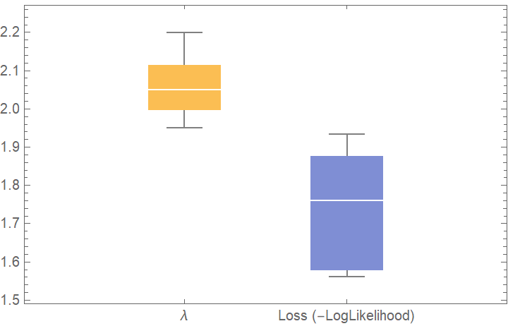
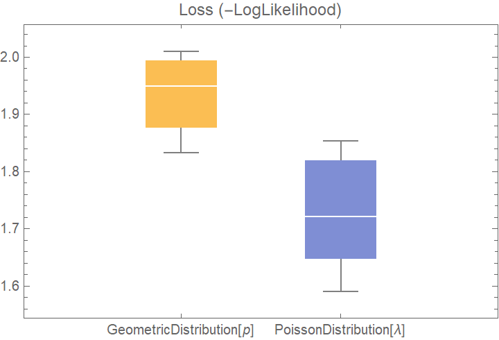
![dists = {GeometricDistribution[p], PoissonDistribution[\[Lambda]]};
val2 = ResourceFunction["CrossValidateModel"][data, dists];
BoxWhiskerChart[{Merge[val2[[All, "ValidationResult"]], Identity]}, "Outliers", ChartLabels -> Automatic, PlotLabel -> "Loss (-LogLikelihood)"]](https://www.wolframcloud.com/obj/resourcesystem/images/27b/27b02800-4e9d-4ff6-8a0e-46bbb178d668/2-1-0/741ebc6fa22d43ef.png)
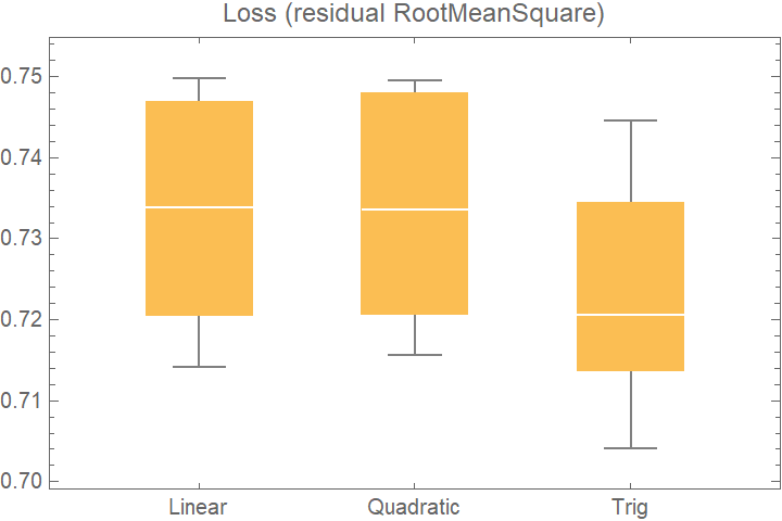
![data = Flatten[
Table[{x, y, Sin[x + y] + RandomVariate[NormalDistribution[0, 0.2]]}, {x, -5, 5, 0.2}, {y, -5, 5, 0.2}], 1];
crossVal = ResourceFunction["CrossValidateModel"][
data,
<|
"Linear" -> Function[LinearModelFit[#, {x, y}, {x, y}]],
"Quadratic" -> Function[LinearModelFit[#, {x, y, x y, x^2, y^2}, {x, y}]],
"Trig" -> Function[LinearModelFit[#, {Sin[x], Cos[y]}, {x, y}]]
|>
];
BoxWhiskerChart[
Merge[crossVal[[All, "ValidationResult"]], Identity], "Outliers", ChartLabels -> Automatic, PlotLabel -> "Loss (residual RootMeanSquare)"]](https://www.wolframcloud.com/obj/resourcesystem/images/27b/27b02800-4e9d-4ff6-8a0e-46bbb178d668/2-1-0/76eab668be11fd05.png)
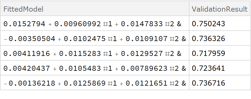
![crossVal = ResourceFunction["CrossValidateModel"][
data,
Function[Fit[#, {1, x, y}, {x, y}, "Function"]]
];
Dataset[crossVal]](https://www.wolframcloud.com/obj/resourcesystem/images/27b/27b02800-4e9d-4ff6-8a0e-46bbb178d668/2-1-0/7189ee7387e5ca8d.png)
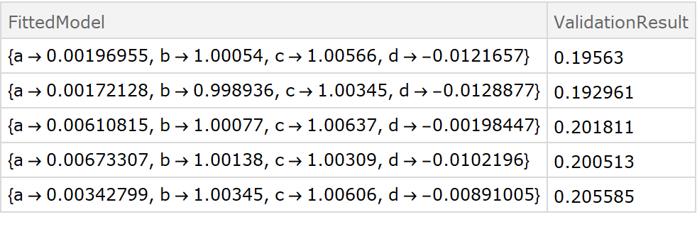
![fitExpression = a + Sin[d + b x + c y];
crossVal = ResourceFunction["CrossValidateModel"][
data,
Function[FindFit[#, fitExpression, {a, b, c, d}, {x, y}]],
"ValidationFunction" -> {
Automatic,
{(* specify the fit expression and the ind*) fitExpression,
{x, y}
}
}
];
Dataset[crossVal]](https://www.wolframcloud.com/obj/resourcesystem/images/27b/27b02800-4e9d-4ff6-8a0e-46bbb178d668/2-1-0/5b79c73790596b72.png)
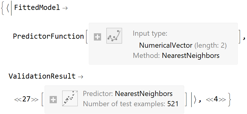
![data = Flatten[
Table[{x, y, Sin[x + y] + RandomVariate[NormalDistribution[0, 0.2]]}, {x, -5, 5, 0.2}, {y, -5, 5, 0.2}], 1];
ResourceFunction["CrossValidateModel"][
data[[All, {1, 2}]] -> data[[All, 3]], Function[Predict[#, TimeGoal -> 5]]] // Short](https://www.wolframcloud.com/obj/resourcesystem/images/27b/27b02800-4e9d-4ff6-8a0e-46bbb178d668/2-1-0/3b7b6e2219bc3d3c.png)
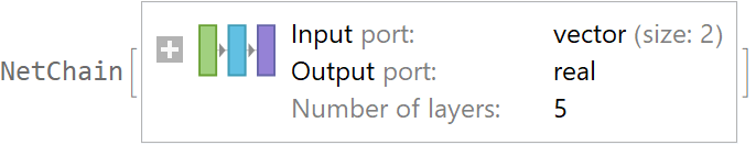
![data = Flatten[
Table[{x, y, Sin[x + y] + RandomVariate[NormalDistribution[0, 0.2]]}, {x, -5, 5, 0.2}, {y, -5, 5, 0.2}], 1];
net = NetTrain[NetChain[{10, Ramp, 10, Ramp, LinearLayer[]}], data[[All, {1, 2}]] -> data[[All, 3]], TimeGoal -> 5]](https://www.wolframcloud.com/obj/resourcesystem/images/27b/27b02800-4e9d-4ff6-8a0e-46bbb178d668/2-1-0/4f712060baf26db1.png)
![val = ResourceFunction["CrossValidateModel"][
data[[All, {1, 2}]] -> data[[All, 3]], Function[NetTrain[net, #, All, TimeGoal -> 5]]];
val[[All, "ValidationResult"]]](https://www.wolframcloud.com/obj/resourcesystem/images/27b/27b02800-4e9d-4ff6-8a0e-46bbb178d668/2-1-0/70376a100efda1dd.png)
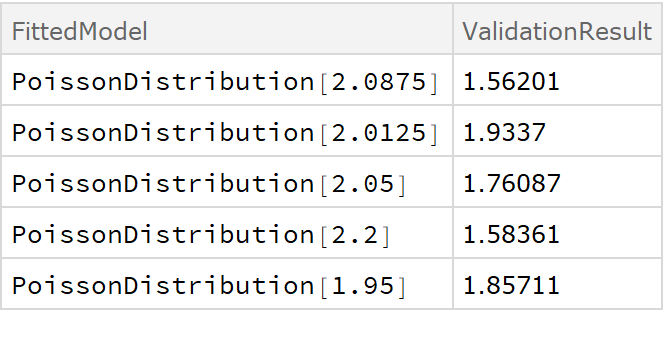
![crossVal = ResourceFunction["CrossValidateModel"][
RandomVariate[PoissonDistribution[2], 100], PoissonDistribution[\[Lambda]],
Method -> {"KFold", "Folds" -> 10, "Runs" -> 4}
];
Length[crossVal]](https://www.wolframcloud.com/obj/resourcesystem/images/27b/27b02800-4e9d-4ff6-8a0e-46bbb178d668/2-1-0/3694b5727aed9bb8.png)
![crossVal = ResourceFunction["CrossValidateModel"][
RandomVariate[PoissonDistribution[2], 100], PoissonDistribution[\[Lambda]],
Method -> "LeaveOneOut",
"ParallelQ" -> True
];
Length[crossVal]](https://www.wolframcloud.com/obj/resourcesystem/images/27b/27b02800-4e9d-4ff6-8a0e-46bbb178d668/2-1-0/651f8c36d361e535.png)
![crossVal = ResourceFunction["CrossValidateModel"][
RandomVariate[PoissonDistribution[2], 100], PoissonDistribution[\[Lambda]],
Method -> {"RandomSubSampling",
"Runs" -> 100,
ValidationSet -> Scaled[0.1], (* This illustrates how the default "SamplingFunction" can be replicated as an explicit Function *) "SamplingFunction" -> Function[{nData, nVal},(* The sampling function accepts the number of data points and number of validation points as inputs*) AssociationThread[(*The output should be an Association with 2 lists of indices 1 \[LessEqual] i \[LessEqual] nData *)
{"TrainingSet", "ValidationSet"},
TakeDrop[RandomSample[Range[nData]], nData - nVal]
]
]
},
"ParallelQ" -> True
] // Short](https://www.wolframcloud.com/obj/resourcesystem/images/27b/27b02800-4e9d-4ff6-8a0e-46bbb178d668/2-1-0/57d6fc06b6330369.png)
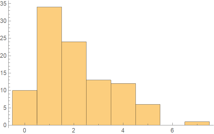
![bootStrap = ResourceFunction["CrossValidateModel"][
RandomVariate[PoissonDistribution[2], 100], PoissonDistribution[\[Lambda]],
Method -> {"BootStrap", "Runs" -> 1000, "BootStrapSize" -> Scaled[1]},
"ParallelQ" -> True
];
BoxWhiskerChart[bootStrap[[All, "FittedModel", 1]], "Outliers", ChartLabels -> {"\[Lambda]"}]](https://www.wolframcloud.com/obj/resourcesystem/images/27b/27b02800-4e9d-4ff6-8a0e-46bbb178d668/2-1-0/16bc9c07a0c20636.png)

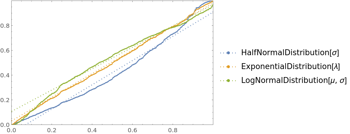
![cdfValues = ResourceFunction["CrossValidateModel"][
RandomVariate[ExponentialDistribution[1], 1000],
{HalfNormalDistribution[\[Sigma]], ExponentialDistribution[\[Lambda]], LogNormalDistribution[\[Mu], \[Sigma]]},
"ValidationFunction" -> Function[{fittedDistribution, validationData},
CDF[fittedDistribution, validationData] (*This should be uniformly distributed if the fit is good *)
]
];
QuantilePlot[Merge[cdfValues[[All, "ValidationResult"]], Flatten], UniformDistribution[], PlotLegends -> Keys[cdfValues[[1, 1]]]]](https://www.wolframcloud.com/obj/resourcesystem/images/27b/27b02800-4e9d-4ff6-8a0e-46bbb178d668/2-1-0/597b21f1e1cedc63.png)
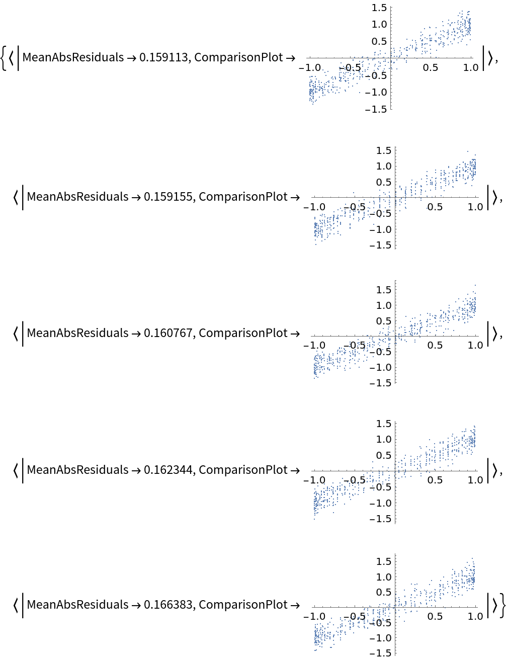
![data = Flatten[
Table[{x, y, Sin[x + y] + RandomVariate[NormalDistribution[0, 0.2]]}, {x, -5, 5, 0.2}, {y, -5, 5, 0.2}], 1];
ResourceFunction["CrossValidateModel"][
data,
Function[
NonlinearModelFit[#, amp*Sin[a x + b y + c] + d, {amp, a, b, c, d}, {x, y}]],
"ValidationFunction" -> {Automatic,
Function[{fittedVals, trueVals}, <|
"MeanAbsResiduals" -> Mean[Abs[fittedVals - trueVals]],
"ComparisonPlot" -> ListPlot[SortBy[First]@Transpose[{fittedVals, trueVals}]]
|>
]
}
][[All, "ValidationResult"]]](https://www.wolframcloud.com/obj/resourcesystem/images/27b/27b02800-4e9d-4ff6-8a0e-46bbb178d668/2-1-0/7babc98d98f52458.png)
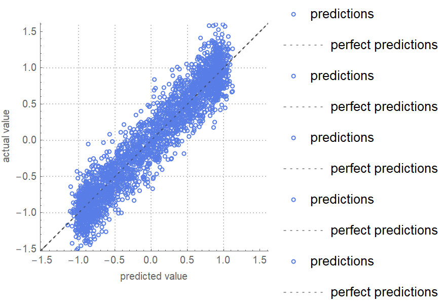
![data = Flatten[
Table[{x, y, Sin[x + y] + RandomVariate[NormalDistribution[0, 0.2]]}, {x, -5, 5, 0.2}, {y, -5, 5, 0.2}], 1];
ResourceFunction["CrossValidateModel"][
data[[All, {1, 2}]] -> data[[All, 3]],
Function[Predict[#, TimeGoal -> 5]],
"ValidationFunction" -> {Automatic, "ComparisonPlot"}
][[All, "ValidationResult"]] // Show](https://www.wolframcloud.com/obj/resourcesystem/images/27b/27b02800-4e9d-4ff6-8a0e-46bbb178d668/2-1-0/20e0c10d48c5f152.png)
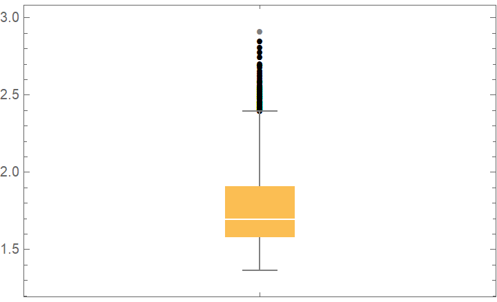
![data = Flatten[
Table[{x, y, Sin[x + y] + RandomVariate[NormalDistribution[0, 0.2]]}, {x, -5, 5, 0.2}, {y, -5, 5, 0.2}], 1];
net = NetTrain[NetChain[{10, Ramp, 10, Ramp, LinearLayer[]}], data[[All, {1, 2}]] -> data[[All, 3]], TimeGoal -> 5];
ResourceFunction["CrossValidateModel"][
data[[All, {1, 2}]] -> data[[All, 3]], Function[NetTrain[net, #, All, TimeGoal -> 5]],
"ValidationFunction" -> {Automatic, "MeanDeviation"}
][[All, "ValidationResult"]]](https://www.wolframcloud.com/obj/resourcesystem/images/27b/27b02800-4e9d-4ff6-8a0e-46bbb178d668/2-1-0/2c27b9ff6d5f9388.png)

![crossVal = ResourceFunction["CrossValidateModel"][
RandomVariate[PoissonDistribution[2], 100], PoissonDistribution[\[Lambda]],
Method -> {"KFold", "Folds" -> 10, "Runs" -> 500},
"ParallelQ" -> {True, Method -> "CoarsestGrained"}
];
BoxWhiskerChart[crossVal[[All, "ValidationResult"]], "Outliers"]](https://www.wolframcloud.com/obj/resourcesystem/images/27b/27b02800-4e9d-4ff6-8a0e-46bbb178d668/2-1-0/26004aa8e16d9f5a.png)
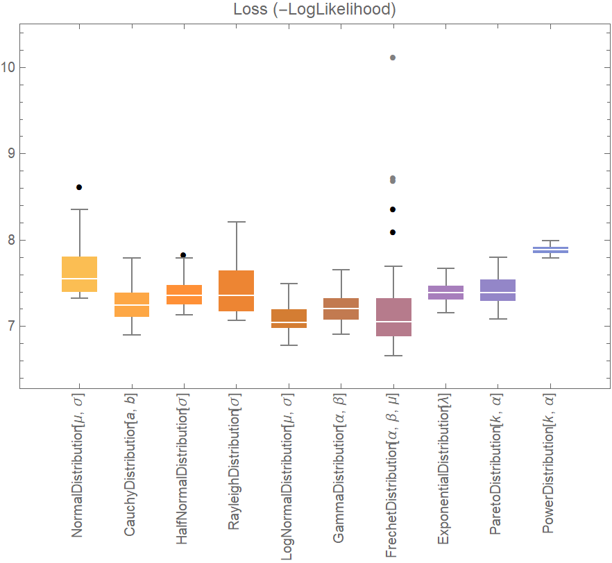
![data = ExampleData[{"Statistics", "RiverLengths"}];
dists = {
NormalDistribution[\[Mu], \[Sigma]], CauchyDistribution[a, b], HalfNormalDistribution[\[Sigma]],
RayleighDistribution[\[Sigma]], LogNormalDistribution[\[Mu], \[Sigma]],
GammaDistribution[\[Alpha], \[Beta]], FrechetDistribution[\[Alpha], \[Beta], \[Mu]], ExponentialDistribution[\[Lambda]], ParetoDistribution[k, \[Alpha]], PowerDistribution[k, \[Alpha]]
};
val = ResourceFunction["CrossValidateModel"][data, dists,
Method -> {"KFold", "Runs" -> 10},
"ParallelQ" -> True
];
BoxWhiskerChart[{Merge[val[[All, "ValidationResult"]], Identity]}, "Outliers", ChartLabels -> Thread@Rotate[dists, 90 Degree], PlotLabel -> "Loss (-LogLikelihood)"]](https://www.wolframcloud.com/obj/resourcesystem/images/27b/27b02800-4e9d-4ff6-8a0e-46bbb178d668/2-1-0/23d22327aad27cde.png)
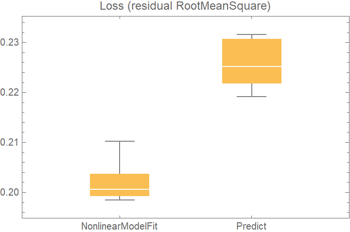
![data = Flatten[
Table[{x, y} -> Sin[x + y] + RandomVariate[NormalDistribution[0, 0.2]], {x, -5, 5, 0.2}, {y, -5, 5, 0.2}], 1];
crossVal = ResourceFunction["CrossValidateModel"][
data,
<| "NonlinearModelFit" -> Function[
NonlinearModelFit[Append @@@ #, Sin[a x + b y + c], {a, b, c}, {x, y}]],
"Predict" -> Function[Predict[#]]
|>
,
"ValidationFunction" -> <|
(* the default validation function will be used for NonlinearModelFit, so it does not need to be specified *) "Predict" -> {Automatic, "StandardDeviation"}
|>,
"ParallelQ" -> True
];
BoxWhiskerChart[
Merge[crossVal[[All, "ValidationResult"]], Identity], "Outliers", ChartLabels -> Automatic, PlotLabel -> "Loss (residual RootMeanSquare)"]](https://www.wolframcloud.com/obj/resourcesystem/images/27b/27b02800-4e9d-4ff6-8a0e-46bbb178d668/2-1-0/6a097c7dea980521.png)