Wolfram Function Repository
Instant-use add-on functions for the Wolfram Language
Function Repository Resource:
Compute the curvature of a curve
ResourceFunction["Curvature"][c,t] computes the curvature of curve c parametrized by t. |
Plot the twisted cubic curve:
| In[1]:= |
| Out[1]= | 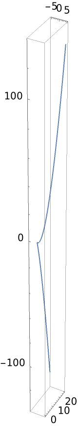 |
Compute the curvature of the twisted cubic curve:
| In[2]:= |
| Out[2]= |
Compute the torsion with the resource function CurveTorsion:
| In[3]:= |
| Out[3]= |
Plot them:
| In[4]:= |
| Out[4]= | 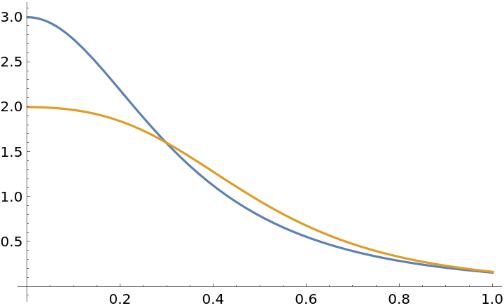 |
For a plane curve, the curvature and torsion are the same:
| In[5]:= |
| Out[5]= |
| In[6]:= |
| Out[6]= |
Make a plot:
| In[7]:= |
| Out[7]= | 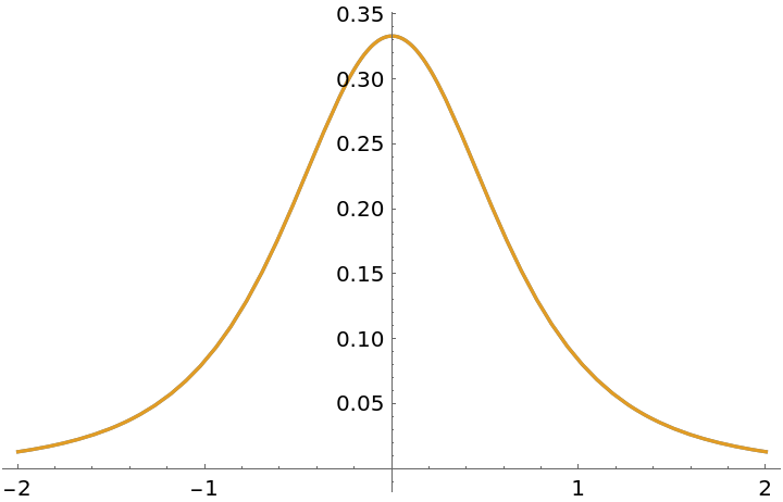 |
A curve that is qualitatively similar to a torus knot:
| In[8]:= |
Plot the knot:
| In[9]:= |
| Out[9]= | 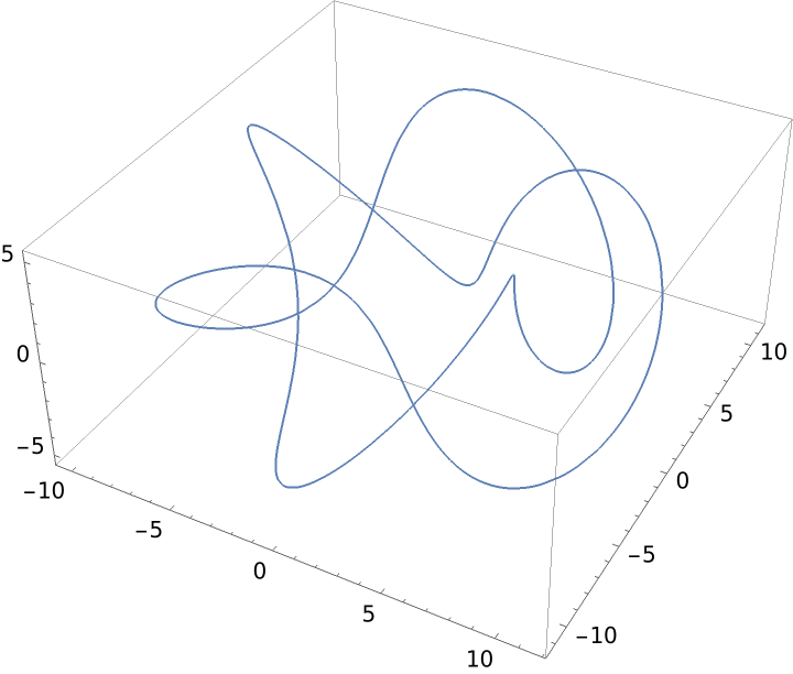 |
Find the curvature:
| In[10]:= |
| Out[10]= |
Plot it:
| In[11]:= |
| Out[11]= | 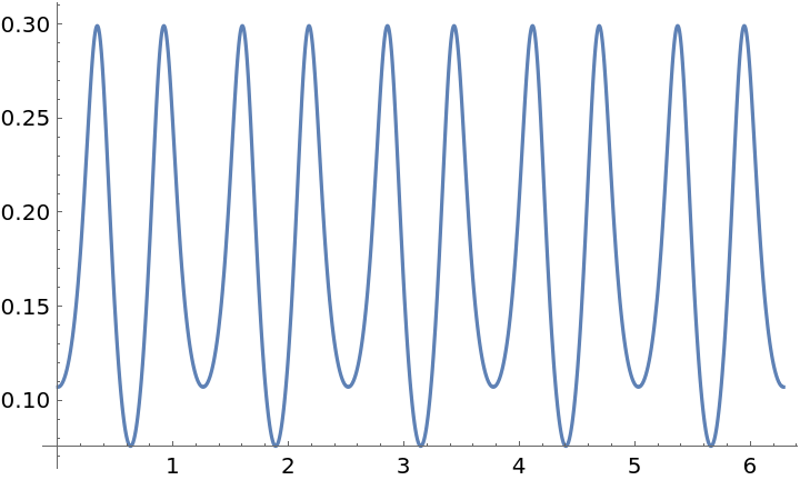 |
Find the torsion with the resource function CurveTorsion:
| In[12]:= |
| Out[12]= |  |
Plot the torsion:
| In[13]:= |
| Out[13]= | 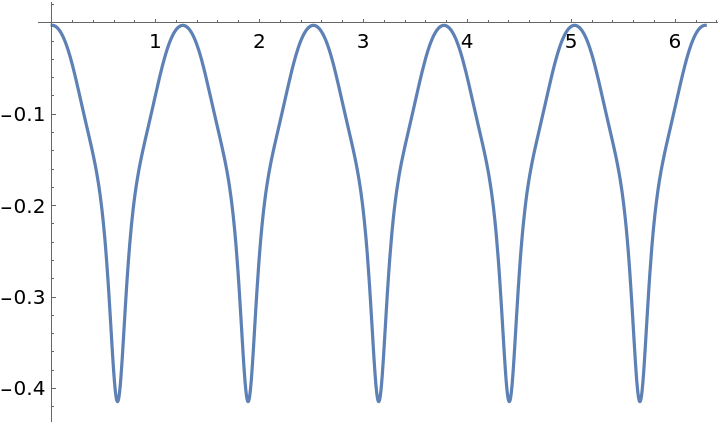 |
Define a loxodrome:
| In[14]:= |
| In[15]:= |
| Out[15]= |
Compute its curvature:
| In[16]:= |
| Out[16]= |  |
Plot the curvature:
| In[17]:= |
| Out[17]= | 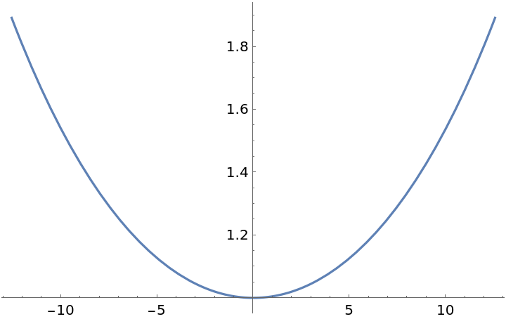 |
A curve colored according to its curvature value:
| In[18]:= | ![range = Last[PlotRange /. AbsoluteOptions[gr, PlotRange]];
Show[ParametricPlot3D[loxodromes[1, 0.1], {u, -4 Pi, 4 Pi}, ColorFunction -> Function[{x, y, z, u, v}, ColorData["Rainbow"][Rescale[cur, range]]], ColorFunctionScaling -> False, PlotStyle -> Thickness[0.01]], Graphics3D[{Opacity[0.2], Sphere[]}]]](https://www.wolframcloud.com/obj/resourcesystem/images/8bf/8bf8786e-87ba-416d-b7e8-401dd370e750/63b639d0b662bb01.png) |
| Out[18]= | 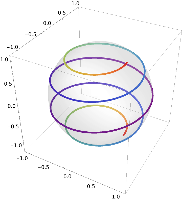 |
A plane curve in polar coordinates:
| In[19]:= |
| In[20]:= |
| Out[20]= |
Plot it:
| In[21]:= |
| Out[21]= | 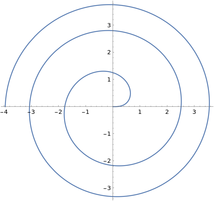 |
The curvature:
| In[22]:= |
| Out[22]= |
The curvature of a circle:
| In[23]:= |
| Out[23]= |
The curvature of the Cornu spiral:
| In[24]:= |
| Out[24]= |
Define a conical spiral:
| In[25]:= |
| Out[25]= |
Compute the curvature:
| In[26]:= |
| Out[26]= |
Definition of a unit speed helix:
| In[27]:= | ![uhelix = {a Cos[t/Sqrt[a^2 + b^2]], a Sin[t/Sqrt[a^2 + b^2]], (b t)/
Sqrt[a^2 + b^2]};](https://www.wolframcloud.com/obj/resourcesystem/images/8bf/8bf8786e-87ba-416d-b7e8-401dd370e750/6bab384b4ca5ef43.png) |
The curvature:
| In[28]:= |
| Out[28]= |
The tangent vector, via the resource function TangentVector:
| In[29]:= |
| Out[29]= |  |
Derivative of the tangent vector:
| In[30]:= |
| Out[30]= |
The normal vector, via the resource function NormalVector:
| In[31]:= |
| Out[31]= |
The curvature times the normal vector is equal to the derivative of the tangent vector:
| In[32]:= |
| Out[32]= |
The torsion, via the resource function CurveTorsion:
| In[33]:= |
| Out[33]= |
In the Frenet–Serret system, the curvature and the torsion are the first two quantities:
| In[34]:= |
| Out[34]= |  |
This work is licensed under a Creative Commons Attribution 4.0 International License