Wolfram Function Repository
Instant-use add-on functions for the Wolfram Language
Function Repository Resource:
Compute the normal vector of a curve
ResourceFunction["NormalVector"][c,t] computes the normal vector for a curve c parametrized by t. |
A unit speed helix:
| In[1]:= | ![uhelix = {a Cos[t/Sqrt[a^2 + b^2]], a Sin[t/Sqrt[a^2 + b^2]], (b t)/
Sqrt[a^2 + b^2]};](https://www.wolframcloud.com/obj/resourcesystem/images/d24/d24d18da-02d0-4a45-b45d-f8f8de682bcb/73c9483671f5623f.png) |
Compute the normal vector:
| In[2]:= |
| Out[2]= |
The normal vector of a figure-eight curve:
| In[3]:= |
| Out[3]= |
| In[4]:= | ![Manipulate[
ParametricPlot[{Cos[t], Sin[t] Cos[t]}, {t, 0, 2 \[Pi]}, Epilog -> Arrow[{{Cos[tf], Sin[tf] Cos[
tf]}, ({Cos[t], Sin[t] Cos[t]} + .3 ResourceFunction[
"NormalVector"][{Cos[t], Sin[t] Cos[t]}, t] /. t -> tf)}], PlotRange -> {{-1.3, 1.3}, {-.8, .8}}], {tf, .1, 2 \[Pi]}]](https://www.wolframcloud.com/obj/resourcesystem/images/d24/d24d18da-02d0-4a45-b45d-f8f8de682bcb/6168f01dfaf931d7.png) |
| Out[4]= | 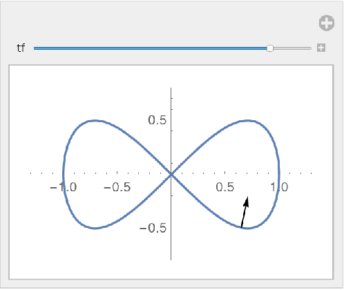 |
Plot a set of normal vectors:
| In[5]:= | ![ParametricPlot[{Cos[t], Sin[t] Cos[t]}, {t, 0, 2 \[Pi]}, Epilog -> Table[Line[{{Cos[tf], Sin[tf] Cos[
tf]}, ({Cos[t], Sin[t] Cos[t]} + .5 ResourceFunction[
"NormalVector"][{Cos[t], Sin[t] Cos[t]}, t] /. t -> tf)}], {tf, 0, 2 \[Pi], .1}], PlotRange -> {{-1.5, 1.3}, {-1, 1}}]](https://www.wolframcloud.com/obj/resourcesystem/images/d24/d24d18da-02d0-4a45-b45d-f8f8de682bcb/1fa414bc2d61c4b5.png) |
| Out[5]= | 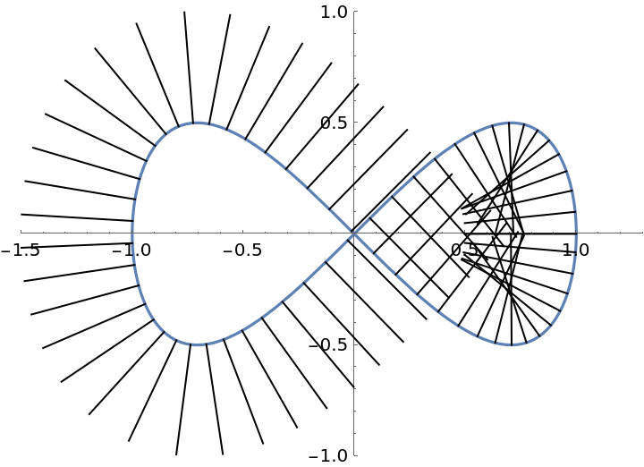 |
Define a helix curve:
| In[6]:= |
Compute the normal vector:
| In[7]:= |
| Out[7]= |
The binormal vector, via the resource function BinormalVector:
| In[8]:= |
| Out[8]= |
The normal plane is spanned by the normal vector and the binormal vector. It can be computed with the resource function NormalPlane:
| In[9]:= |
| Out[9]= |
The normal plane and the normal vector along the helix:
| In[10]:= | ![Manipulate[
Show[ParametricPlot3D[helix, {t, 0, 3}], Graphics3D[{Arrow[{helix, helix + {-Cos[t], -Sin[t], 0}}], Opacity[.5], ResourceFunction[
ResourceObject[<|{"Name" -> "NormalPlane", "ShortName" -> "NormalPlane", "UUID" -> "e083b2e5-d843-4dc2-98e5-9a20518341ee", "ResourceType" -> "Function", "Version" -> "1.0.0", "Description" -> "Compute the normal plane of a space curve", "RepositoryLocation" -> URL[
"https://www.wolframcloud.com/objects/resourcesystem/api/1.0"], "SymbolName" -> "FunctionRepository`$495e9b14e5184131aa3c629c6d3c8005`NormalPlane", "FunctionLocation" -> CloudObject[
"https://www.wolframcloud.com/obj/a318e75b-f17d-4c12-bda1-8414ee7e1565"]}|>, {ResourceSystemBase -> Automatic}]][helix, t]} /. t -> tf], PlotRange -> {{-1, 1}, {-1, 1}, {-1, 3}}], {{tf, 1}, 0, 3}]](https://www.wolframcloud.com/obj/resourcesystem/images/d24/d24d18da-02d0-4a45-b45d-f8f8de682bcb/627c997913ab5450.png) |
| Out[10]= | 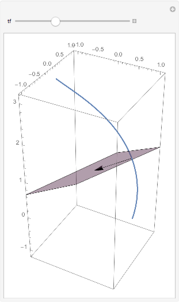 |
The definition of Viviani's curve:
| In[11]:= |
| Out[11]= |
Plot the curve:
| In[12]:= |
| Out[12]= | 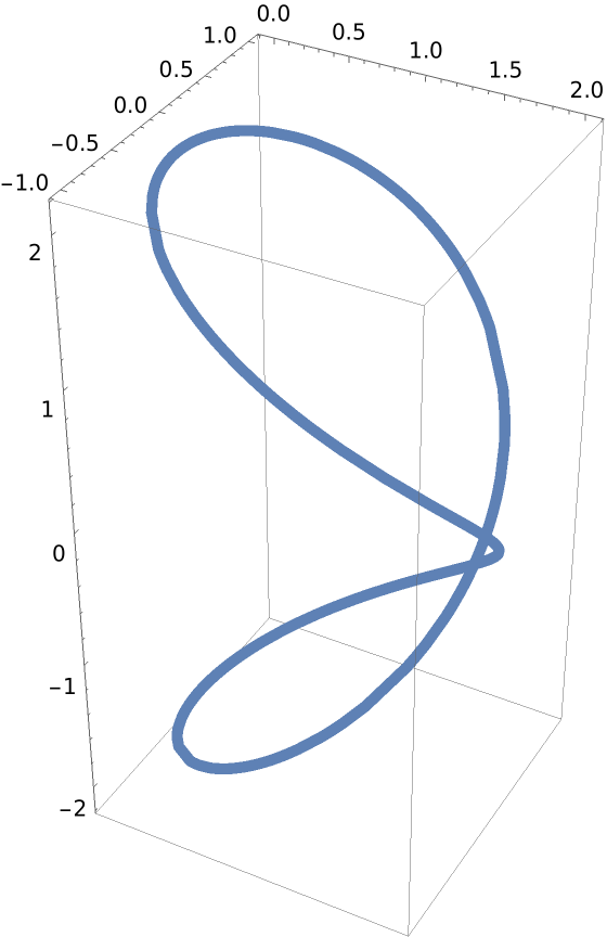 |
The normal surface associated to a curve is generated by its normal vector field. It can be computed with the resource function NormalSurface:
| In[13]:= |
| Out[13]= |  |
Plot the normal surface:
| In[14]:= |
| Out[14]= | 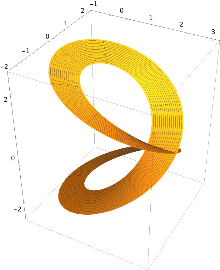 |
A unit speed helix:
| In[15]:= | ![uhelix = {a Cos[t/Sqrt[a^2 + b^2]], a Sin[t/Sqrt[a^2 + b^2]], (b t)/
Sqrt[a^2 + b^2]};](https://www.wolframcloud.com/obj/resourcesystem/images/d24/d24d18da-02d0-4a45-b45d-f8f8de682bcb/3da3b8d8df2c213f.png) |
Compute the normal vector:
| In[16]:= |
| Out[16]= |
Compute the curvature with the resource function Curvature:
| In[17]:= |
| Out[17]= |
Compute the torsion with the resource function CurveTorsion:
| In[18]:= |
| Out[18]= |
Compute the tangent vector with the resource function TangentVector:
| In[19]:= |
| Out[19]= |  |
Compute the binormal vector with the resource function BinormalVector:
| In[20]:= |
| Out[20]= |  |
Compute the following quantity:
| In[21]:= |
| Out[21]= |  |
The previous expression is the derivative of the normal:
| In[22]:= |
| Out[22]= |  |
Using FrenetSerretSystem, the normal vector is the second entry of the second List:
| In[23]:= |
| Out[23]= |  |
This work is licensed under a Creative Commons Attribution 4.0 International License