Basic Examples (3)
Obtain an approximate piecewise Frobenius solution to a differential equation:
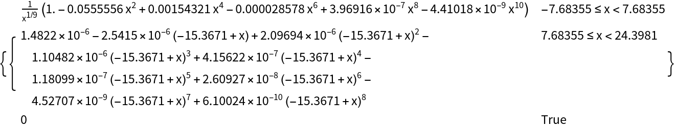
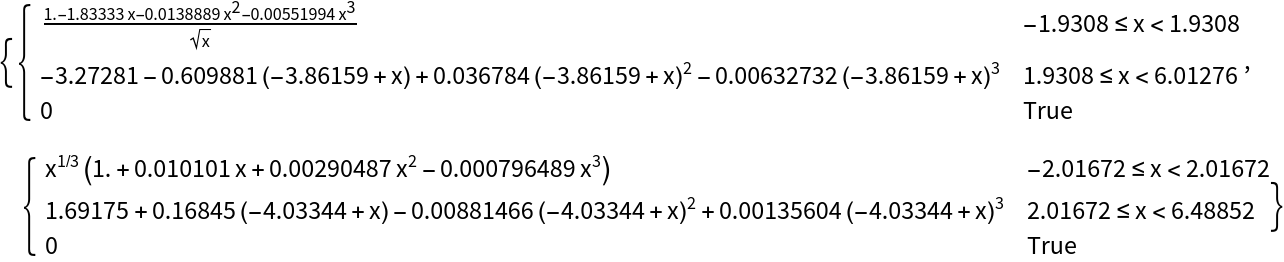
Compute an approximate solution to the ODE 2x2(x+3)2y''+7x(x+3)y'-3y=0 in the domain x∈[0,6] using piecewise Frobenius method:
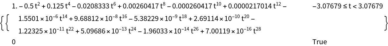
Each of the two solutions is a piecewise Frobenius series. Display the two solutions, omitting for shortness fourth and higher order terms:
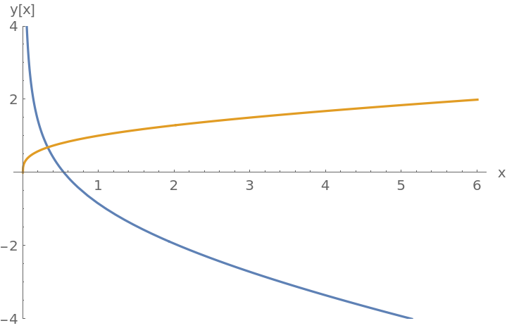
By default, the maximum power of x in each of the Frobenius series is 28 (see Options). Plot the solutions:
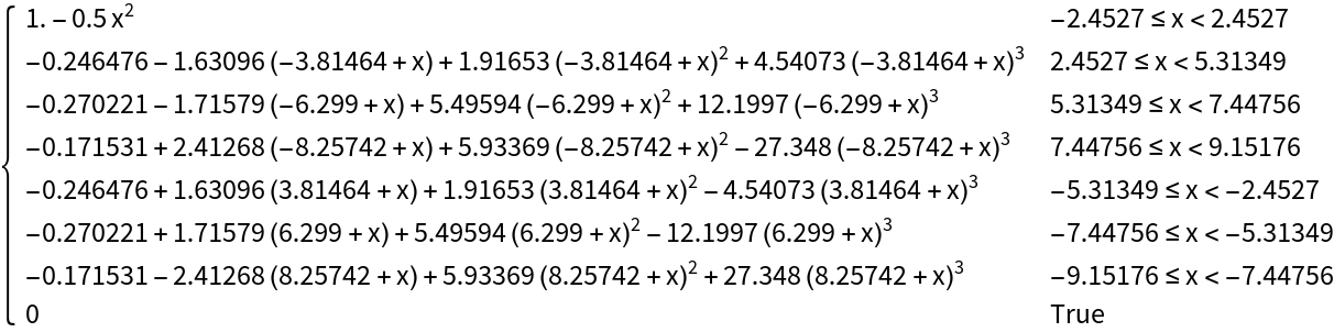
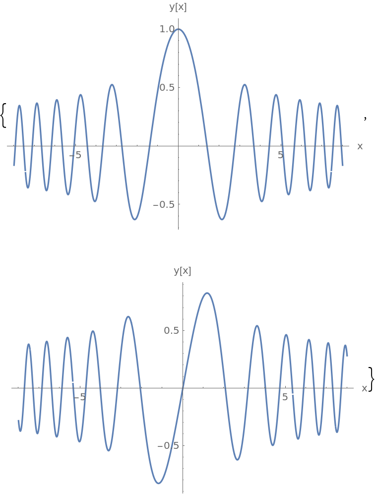
Solve the non-singular ODE y''+(1+x2)y=0 for x between -8 and 8:
Each solution is now a piecewise power series. Display the first solution up to order three:
Solutions to the equation y''+(1+x2)y=0 start oscillating really fast for large x, and to maintain the requested accuracy, FrobeniusPiecewiseDSolve uses many subintervals. Plot the solutions:
Scope (2)
The function can operate with complex numbers:
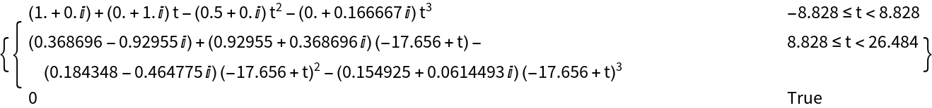
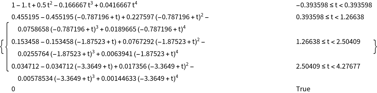
FrobeniusPiecewiseDSolve can be used to solve ODEs of any order. Here, for example, are four linearly independent solutions to y''''[t]+ty[t]=0, with fourth and higher order terms omitted for shortness:
Options (2)
The option "FrobeniusOrder" controls the number of terms in each of the Frobenius series making up the piecewise solution:
FrobeniusPiecewiseDSolve can output solutions of any specified accuracy using the Tolerance option:
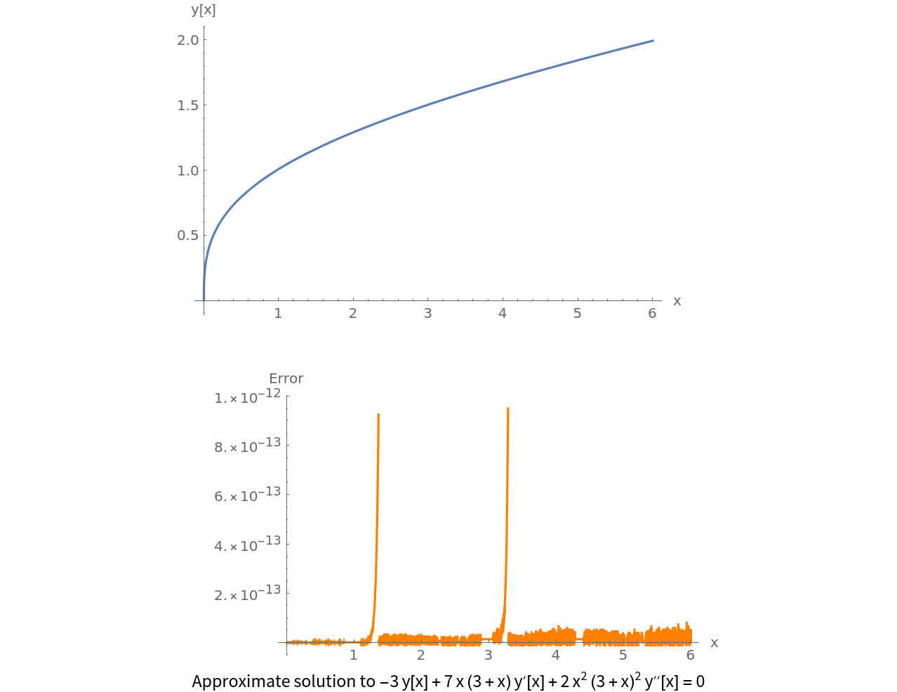
The default value of Tolerance is 10-3. Compute the two linearly independent solutions to 2x2(x+3)2y''+7x(x+3)y'-3y=0 with Tolerance set to 10-12, and then plot the remainder of one of the solutions:
As you can see, error stays below the tolerance of 10-12. This shows that FrobeniusPiecewiseDSolve can be used to quickly compute extremely accurate solutions. Here, the error of an approximate solution  to an ODE of the form L y = 0 is defined to be
 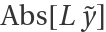 , where L is a linear operator. For the ODE above, the error is
  .
.
Properties and Relations (1)
The time it takes FrobeniusPiecewiseDSolve to compute a solution can be significantly reduced with the help of FrobeniusPiecewiseDSolveFormula:
FrobeniusPiecewiseDSolve first computes a formula and then uses it to calculate the solution. FrobeniusPiecewiseDSolveFormula allows us to compute the formula separately, which can help significantly reduce computation time when an ODE is to be solved repeatedly.
Possible Issues (2)
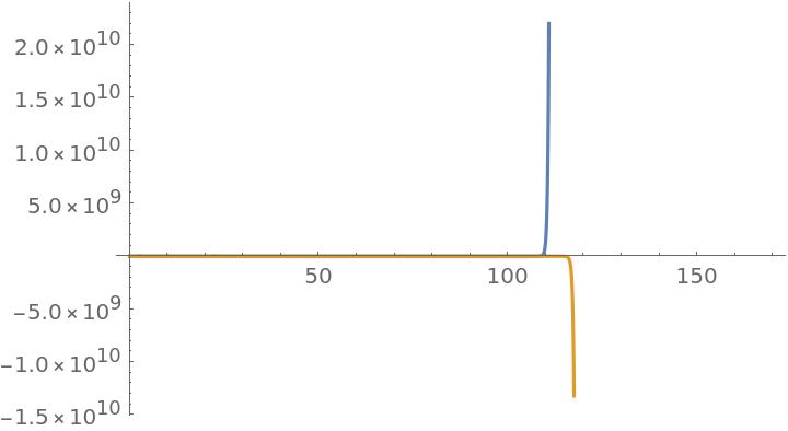
The issues of underflow and overflow may arise if the option "FrobeniusOrder" is made too large. Solve the ODE 2x2(x+3)2y''+7x(x+3)y'-3y=0 with "FrobeniusOrder" set to 200, way above the default value of 28:
As "FrobeniusOrder" gets larger, the function has to compute coefficients aj with larger and larger indexes. And because these coefficients typically decrease with index, at some point the value of the coefficients gets too small for the kernel to process. This makes FrobeniusPiecewiseDSolve underestimate the error of the series solutions, and as a result, it is unable to properly place the subintervals, resulting in an exploding solution:
When solving a given ODE in the region a≤x≤b, FrobeniusPiecewiseDSolve assumes that the ODE either has a singular point at x=a, at x=b, or nowhere between a and b. The algorithm was built on the assumption of continuity. If there is a singular point between a and b, the function will enter an infinite cycle trying to get through the singular point:
This is not a big problem though, as the ODEs we solve on practice either don't have singular points, or the singularities are located in such a way that we wouldn't need to pass through them.

![Block[{eqn = (2 x^2 (x + 3)^2 y''[x] + 7 x (x + 3) y'[x] - 3 y[x]), ncoefs = 40, range = {0, 6}, tol = 10^-12, soln, time, err}, {time, soln} = AbsoluteTiming[
ResourceFunction["FrobeniusPiecewiseDSolve"][eqn == 0, y, x, 0, range, "FrobeniusOrder" -> ncoefs, Tolerance -> tol][[2]]]; Print[Row[{"Computation time: ", Round[1000 * time], " ms"}]]; err = Piecewise@Table[
{Abs[eqn /. (y -> Function[x, Null] /. Null -> reg[[1]])], reg[[2]]},
{reg, soln[[1]]}]; (* for each subregion of the piecewise solution, \
compute the error *) Labeled[Row[{Plot[soln, {x, range[[1]], range[[2]]}, ImageSize -> Medium, AxesLabel -> {"x", "y[x]"}], " ", Plot[err, {x, range[[1]], range[[2]]}, PlotRange -> All, WorkingPrecision -> MachinePrecision, ImageSize -> Medium, AxesLabel -> {"x", "Error"}, PlotStyle -> Orange]}], Row[{"Approximate solution to ", eqn, " = 0"}]]]](https://www.wolframcloud.com/obj/resourcesystem/images/8a0/8a08f410-1a83-4318-9152-ff2d929d12f9/77fcb39698ae8894.png)
![Block[{eqn = (2 x^2 (x + 3)^2 y''[x] + 7 x (x + 3) y'[x] - 3 y[x] == 0), Xmin = 0, Xmax = 6, formula},
formula = FrobeniusPiecewiseDSolveFormula[eqn, y, x, 0];
{
1000 First@
RepeatedTiming@
ResourceFunction["FrobeniusPiecewiseDSolve"][eqn, y, x, 0, {Xmin, Xmax}],
1000 First@
RepeatedTiming@
ResourceFunction["FrobeniusPiecewiseDSolve"][x, 0, {Xmin, Xmax}, formula]
}
]](https://www.wolframcloud.com/obj/resourcesystem/images/8a0/8a08f410-1a83-4318-9152-ff2d929d12f9/0a7c8903ebdfa10f.png)
![TimeConstrained[
ResourceFunction[
"FrobeniusPiecewiseDSolve"][(t - 1) u'[t] + u[t] == 0, u, t, 0, {0, 2}], 3]](https://www.wolframcloud.com/obj/resourcesystem/images/8a0/8a08f410-1a83-4318-9152-ff2d929d12f9/0499185f11be918c.png)