Basic Examples (2) 

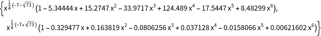
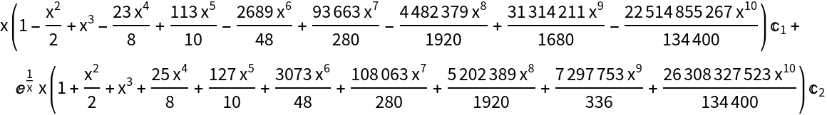
Obtain an order six approximate solution to the ordinary differential equation 2x²y''+9x(x+1)y'-3y=0 using a Frobenius series around the singular point x₀=0:

In[1]:=

Out[1]=

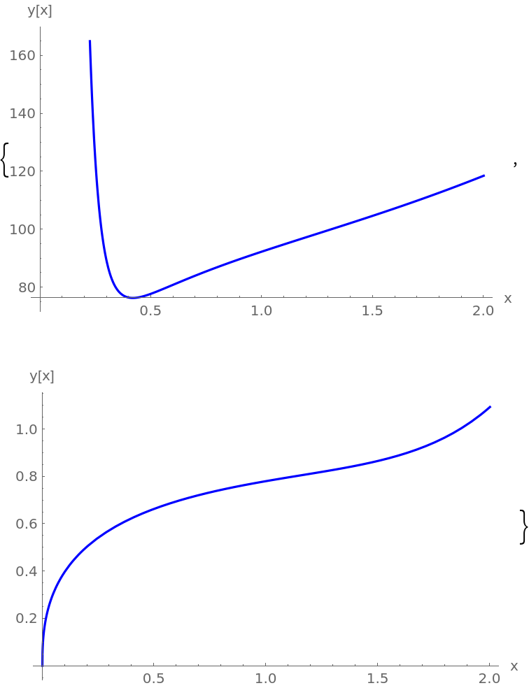
Plot the solutions:

In[2]:=

Out[2]=

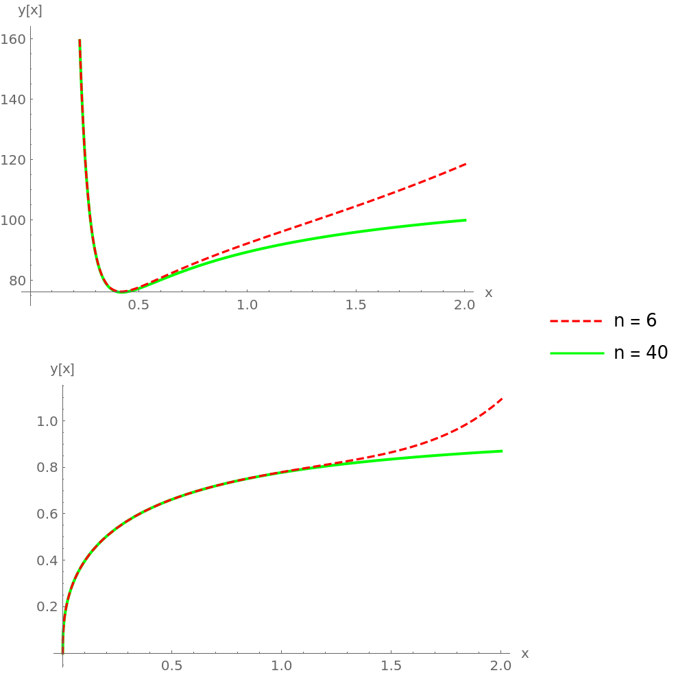
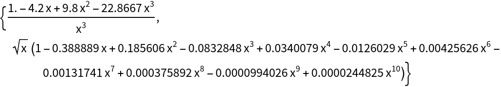
Compute a more accurate solution with n=40 and compare to the previous result:

In[3]:=

In[4]:=

Out[4]=

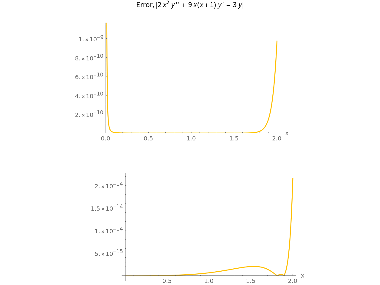
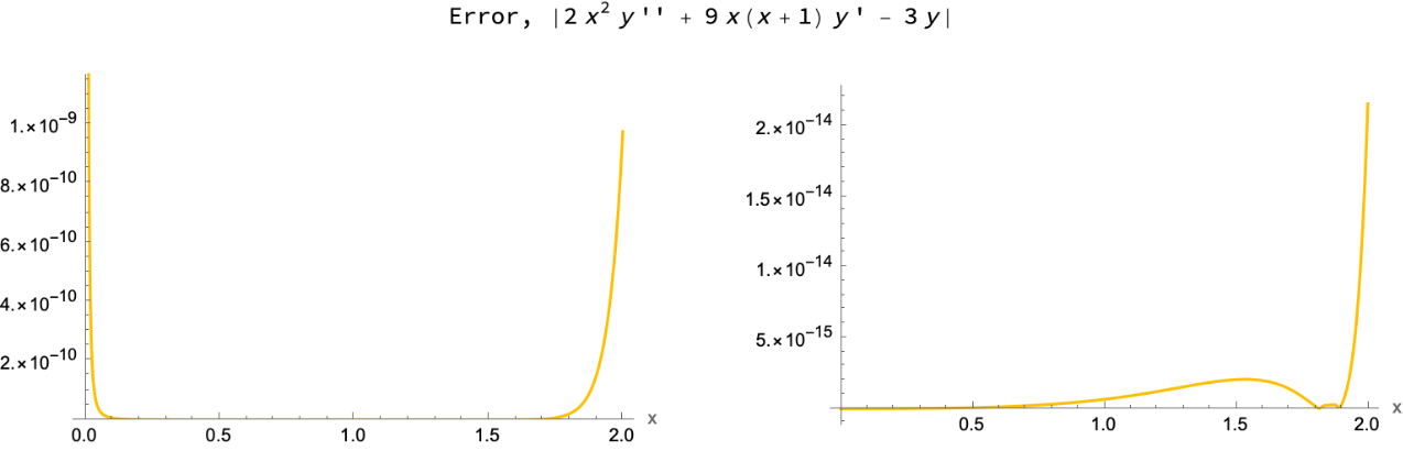
Plot the residuals Abs[x²y''+9x(x+1)y'-3y]:

In[5]:=

Out[5]=

As you can see, the solutions are very accurate. (see Author Notes for more information)

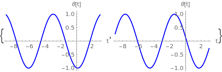
FrobeniusDSolve can also be used to solve equations that don't have singular points. Solve the pendulum equation θ''[t]=-θ[t] near the point t=-3, with n=16:

In[6]:=

Out[6]=

Plot the result:

In[7]:=

Out[7]=

Scope (3) 

The function can operate with complex numbers:

In[8]:=

Out[8]=

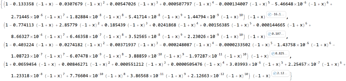
Find a degree 10 approximate solution for the fourth-order ODE (x-1)⁴f''''[x]=x(2+x)f[x]+x²(x-1)²f''[x]-19(x-1)³f'''[x] near the singular point x=1:

In[9]:=

Out[9]=

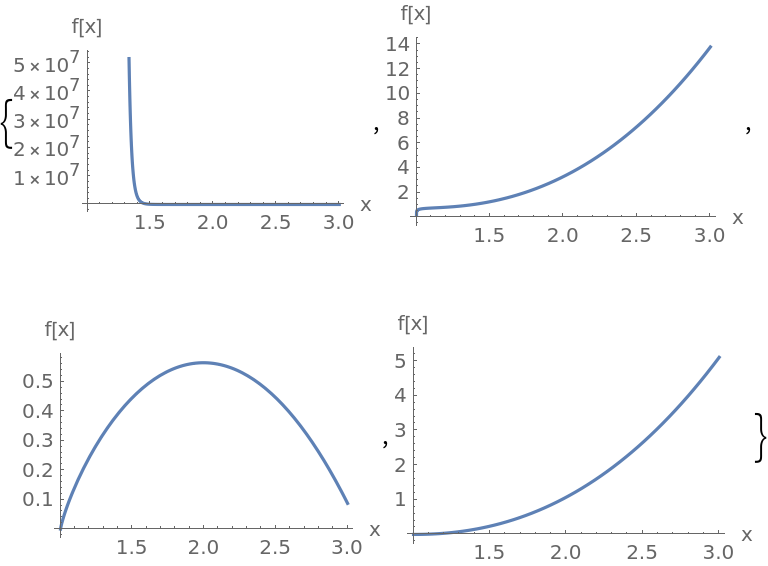
Plot the results:

In[10]:=

Out[10]=

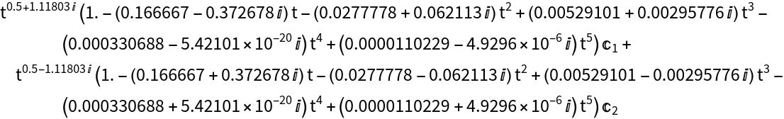
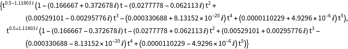
The inputs of the function can be symbolics:

In[11]:=

Out[11]=

In[12]:=

Out[12]=

Options (1) 

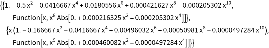
Set "ComputeError" to True to get a formula for the error, defined as the absolute value of the remainder, of a FrobeniusDSolve solution set (see Details and Options):

In[13]:=

Out[13]=

Properties and Relations (5) 

Use AsymptoticDSolveValue to solve the ODE ty''[t]+y[t]=0 near the singular point t=0:

In[14]:=

Out[14]=

Compare to the result from FrobeniusDSolve:

In[15]:=

Out[15]=

Compare timings in milliseconds that FrobeniusDSolve and AsymptoticDSolveValue take to compute the 100th order power series approximation to y''+(1+x²)y=0:

In[16]:=

Out[16]=

FrobeniusDSolve takes roughly 6 milliseconds to compute, while AsymptoticDSolveValue takes about 34. We can reduce computation time even further with the help of the resource function FrobeniusDSolveFormula:

In[17]:=

Out[17]=

When the option "ComputeError" is set to True and FrobeniusDSolveFormula is used, the option "ComputeError" should be switched to True in FrobeniusDSolveFormula, too:

In[18]:=

Out[18]=

Possible Issues (3) 

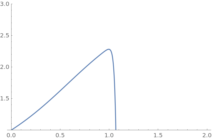
Solutions obtained using Frobenius's method generally only have a finite convergence radius. Try to compute an approximate solution to the ODE (1+x³)y'=y with n=60:

In[19]:=

Out[19]=

The plot looks good for x<1, however, for x>1 the solution starts diverging. To see that, notice that the ODE (1+x³)y'=y demands y' to be positive for x>0, y>0; the plot, however, suddenly goes down at x=1. Besides, the sharpness of the "cliff" looks very suspicious.

Frobenius's method only works near ordinary points or regular singular points. If solution near an irregular singular point is attempted, Frobenius's method would only yield some of the possible solutions or won't be able to find any solutions at all. Consider the ODE x³y''+xy'+(x²-1)y=0 near the singular point x=0:

In[20]:=

Out[20]=

FrobeniusDSolve could only give one of the two linearly independent solutions. The other solution could not be found because it cannot be written in the form 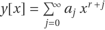, as can be seen with the help of AsymptoticDSolveValue:

In[21]:=

Out[21]=

The parameter n must be at least Z+M, where Z is the order of the ODE and M is the highest power of x (the independent variable). If the ODE is y''''[t]=-(1+t²)y[t], then the order Z=4 and the highest power of t is M=2, so n must be at least 6:

In[22]:=

Out[22]=

Neat Examples (2) 

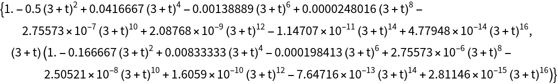
Sometimes, the Frobenius series solution to an ODE consists of a finite number of terms. For example, below are a few examples when the exact solution only has one term in it:

In[23]:=

Out[23]=

In[24]:=

Out[24]=

Sometimes, the solution terminates after a couple terms. While the second of the two solutions below goes on forever, the first one only has four nonzero terms:

In[25]:=

Out[25]=

In[26]:=

Out[26]=