Details and Options
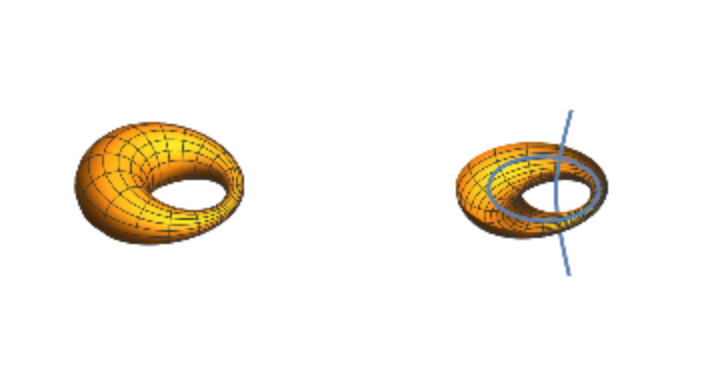
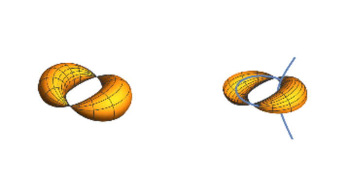
A Dupin cyclide or cyclide of Dupin is any geometric inversion of a standard torus, cylinder or double cone. Charles Dupin discussed his discovery of cyclides in his 1803 dissertation.
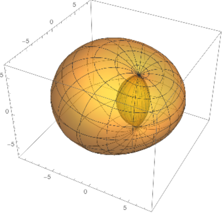
Dupin cyclides are surfaces that are envelopes of spheres. The spheres are then tangent to the cyclides along circles, which are the curvature lines.
The parametrization of elliptic–hyperbolic cyclides is

,
where
a is the semimajor axis,
c is the linear eccentricity of the ellipse and
k is the radius of the generating sphere at the co-vertices of the ellipse
(0,±b), where
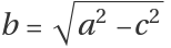
.
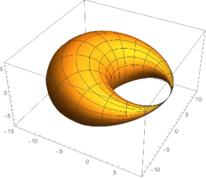
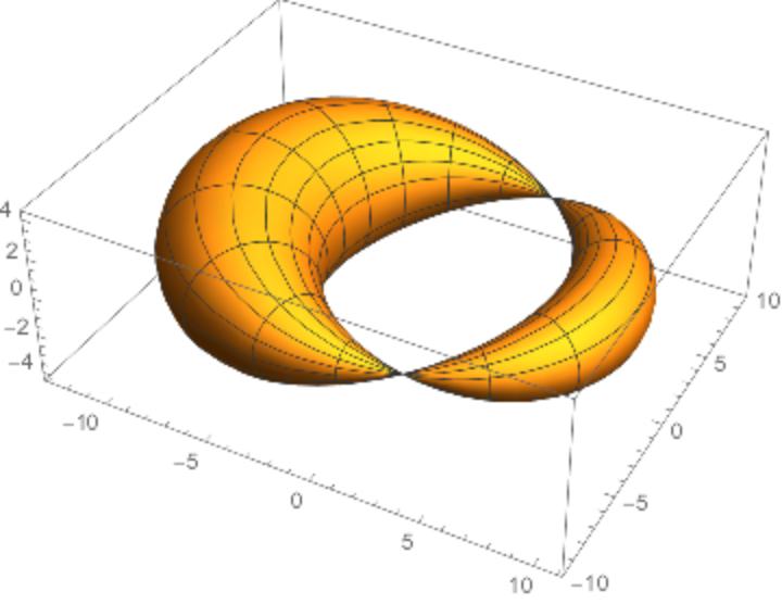
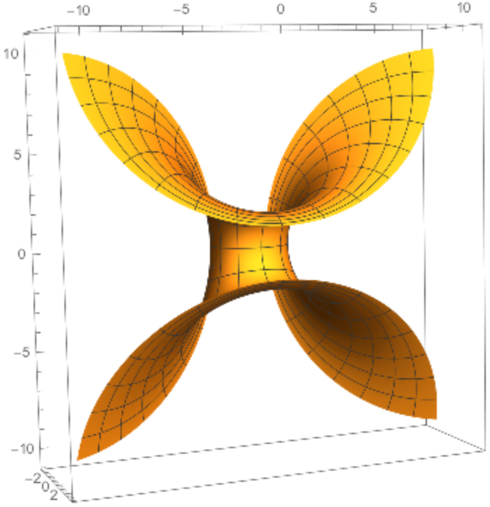
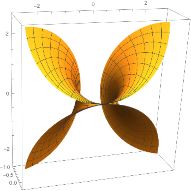
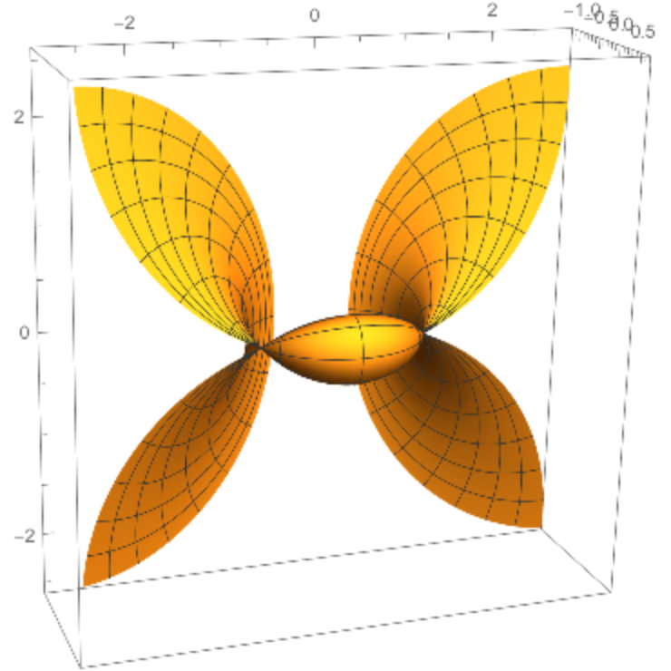
The parametrization of parabolic cyclides is
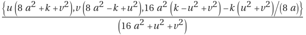
,
where
a determines the shape of the associated parabolas and
k determines the ratio of the diameters of the two holes.
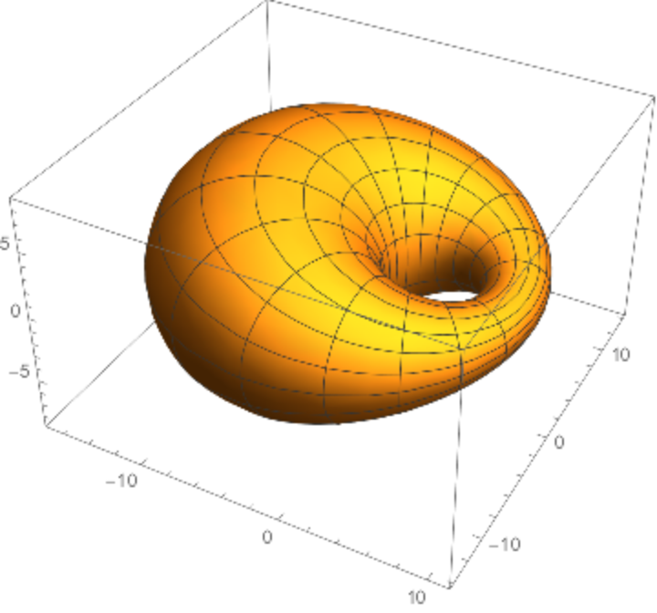
Elliptic–hyperbolic cyclides are a parametrization of Dupin cyclides of radius
k whose focal sets are the ellipse
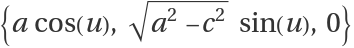
and the hyperbola
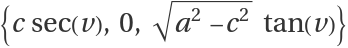
.
Parabolic cyclides are a parametrization of Dupin cyclides of radius k whose focal sets are the parabolas {u,0,-u2/(8 a)+a+k } and {0,v,v2/(8 a)-a-k}.
Dupin cyclides have also been investigated by A. Cayley and J. C. Maxwell.
Dupin cyclides have applications in computer-aided design (CAD).
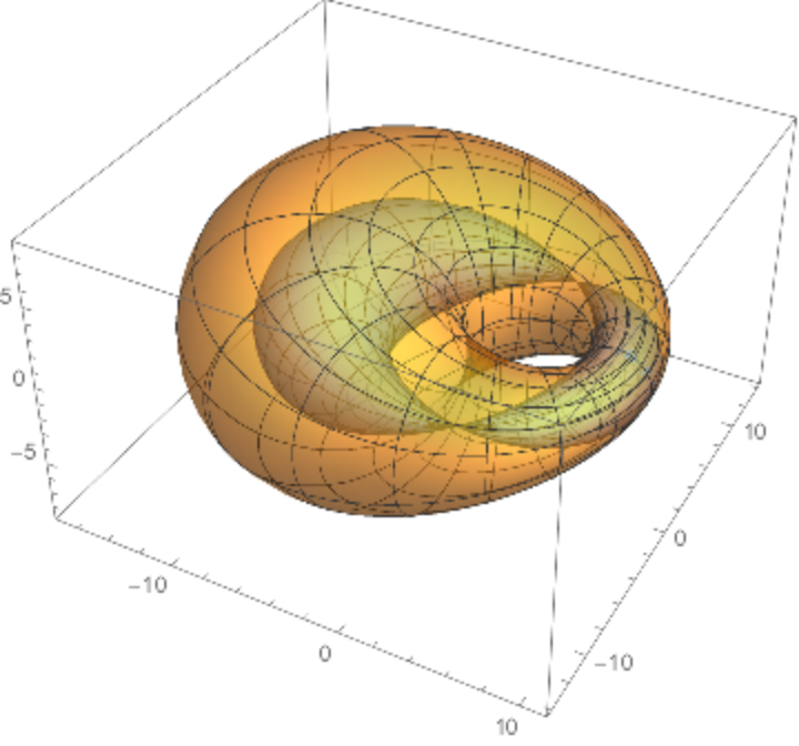
![ParametricPlot3D[
Evaluate[ResourceFunction["Cyclide"][3, 1, 5, {u, v}]], {u, 0, 2 \[Pi]}, {v, 0, 2 \[Pi]}, PlotStyle -> Opacity[.5]]](https://www.wolframcloud.com/obj/resourcesystem/images/738/738c31bb-a402-448f-9fe1-8e66c2b28d5f/1778767b5e2dabb4.png)
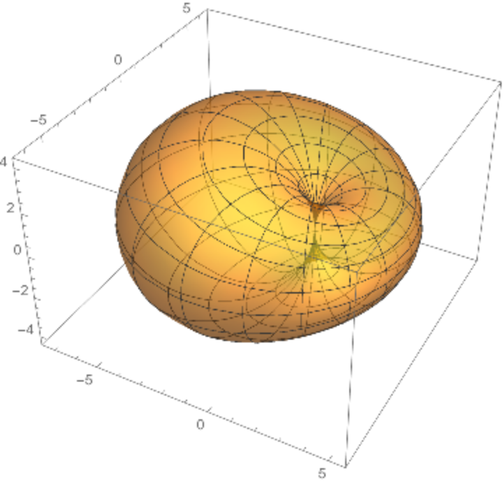
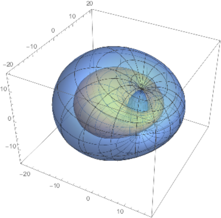
![ParametricPlot3D[
Evaluate[ResourceFunction["Cyclide"][3, 1, 3, {u, v}]], {u, 0, 2 \[Pi]}, {v, 0, 2 \[Pi]}, PlotStyle -> Opacity[.5]]](https://www.wolframcloud.com/obj/resourcesystem/images/738/738c31bb-a402-448f-9fe1-8e66c2b28d5f/19cb4f1b364b4d69.png)
![ParametricPlot3D[
ResourceFunction["Cyclide"][2, 1, {u, v}], {u, -20, 20}, {v, -20, 20}, PlotPoints -> 80, BoxRatios -> {1, 1, .3}]](https://www.wolframcloud.com/obj/resourcesystem/images/738/738c31bb-a402-448f-9fe1-8e66c2b28d5f/0e7f3cf4c15aa519.png)
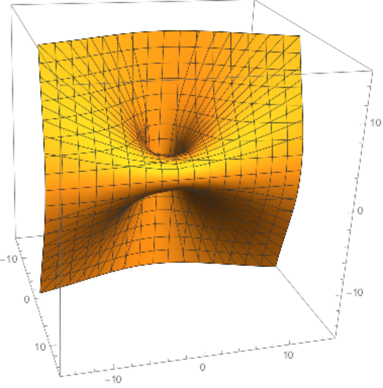
![ParametricPlot3D[
ResourceFunction["Cyclide"][.36, 1., {u, v}], {u, -5, 5}, {v, -5, 5},
PlotPoints -> 80, BoxRatios -> {1, 1, .3}]](https://www.wolframcloud.com/obj/resourcesystem/images/738/738c31bb-a402-448f-9fe1-8e66c2b28d5f/6e1a11cd359826b5.png)
![ParametricPlot3D[
ResourceFunction["Cyclide"][.3, 1.5, {u, v}], {u, -5, 5}, {v, -5, 5},
PlotPoints -> 80, BoxRatios -> {1, 1, .3}]](https://www.wolframcloud.com/obj/resourcesystem/images/738/738c31bb-a402-448f-9fe1-8e66c2b28d5f/4b2f680f4c089244.png)
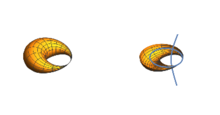
![cycgen[a_, c_, k_, rau_, rav_, opts___] :=
Module[{x, z, \[Alpha], \[Beta]}, x = ResourceFunction["Cyclide"][a, c, k, {u, v}]; z[1] = ParametricPlot3D[x, rau, rav, opts, Boxed -> False, Axes -> False]; \[Alpha][t_] := {a Cos[t], Sqrt[a^2 - c^2] Sin[t],
0}; \[Beta][t_] := {c Sec[t], 0, Sqrt[a^2 - c^2] Tan[t]}; z[2] = ParametricPlot3D[\[Alpha][t], {t, -\[Pi], \[Pi]}]; z[3] = ParametricPlot3D[\[Beta][t], {t, -.499 \[Pi], .499 \[Pi]}]; Show[Array[z, 3], PlotRange -> {{-a - c - k, a + c + k}, {-a - c - k, a + c + k}, {-a - c - k, a + c + k}}]]](https://www.wolframcloud.com/obj/resourcesystem/images/738/738c31bb-a402-448f-9fe1-8e66c2b28d5f/7d3072d7ac485ea4.png)
![x = ResourceFunction["Cyclide"][12, 3, 4.5, {u, v}];
z[1] = ParametricPlot3D[Evaluate[x], {u, 0, 2 \[Pi]}, {v, 0, 2 \[Pi]},
Boxed -> False, Axes -> False, PlotRange -> 19.5];
z[2] = cycgen[12, 3, 4.5, {u, 0, 2 \[Pi]}, {v, -\[Pi], 0}];
GraphicsGrid[{Array[z, 2]}]](https://www.wolframcloud.com/obj/resourcesystem/images/738/738c31bb-a402-448f-9fe1-8e66c2b28d5f/410a38ceedf6a295.png)
![x = ResourceFunction["Cyclide"][8, 4, 0, {u, v}];
z[1] = ParametricPlot3D[Evaluate[x], {u, 0, 2 \[Pi]}, {v, 0, 2 \[Pi]},
Boxed -> False, Axes -> False, PlotRange -> 12];
z[2] = cycgen[8, 4, 0, {u, 0, 2 \[Pi]}, {v, -\[Pi], 0}];
GraphicsGrid[{Array[z, 2]}]](https://www.wolframcloud.com/obj/resourcesystem/images/738/738c31bb-a402-448f-9fe1-8e66c2b28d5f/7674ed20700af301.png)
![Module[{x, z},
x = ResourceFunction["Cyclide"][12, 4, 4, {u, v}];
z[1] = ParametricPlot3D[x // Evaluate,
{u, 0, 2 \[Pi]}, {v, 0, 2 \[Pi]}, Boxed -> False, Axes -> False, PlotRange -> 20];
z[2] = cycgen[12, 4, 4, {u, 0, 2 \[Pi]}, {v, -\[Pi], 0}]; GraphicsGrid[{Array[z, 2]}]
]](https://www.wolframcloud.com/obj/resourcesystem/images/738/738c31bb-a402-448f-9fe1-8e66c2b28d5f/0afa75b3246e9852.png)
![ParametricPlot3D[
Evaluate[{ResourceFunction["Cyclide"][8, 3, 5][u, v], psc}], {u, -\[Pi], \[Pi]}, {v, -\[Pi], \[Pi]}, PlotPoints -> {40, 15}, PlotStyle -> Opacity[.5]]](https://www.wolframcloud.com/obj/resourcesystem/images/738/738c31bb-a402-448f-9fe1-8e66c2b28d5f/7e4b2ac1d260fef7.png)
![ParametricPlot3D[
Evaluate[{ResourceFunction["Cyclide"][8, 3, 5, {u, v}], pscn}], {u, -\[Pi], \[Pi]}, {v, -\[Pi], \[Pi]}, PlotPoints -> {40, 15}, PlotStyle -> Opacity[.5]]](https://www.wolframcloud.com/obj/resourcesystem/images/738/738c31bb-a402-448f-9fe1-8e66c2b28d5f/4cc229b0e51eb546.png)
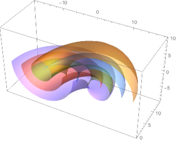
![ParametricPlot3D[
Evaluate[
Table[ResourceFunction["Cyclide"][8, 3, n, {u, v}], {n, -6, 6, 3}]],
{u, 0, \[Pi]}, {v, -\[Pi], 0}, Mesh -> False, PlotPoints -> {40, 15},
PlotStyle -> Opacity[.5]]](https://www.wolframcloud.com/obj/resourcesystem/images/738/738c31bb-a402-448f-9fe1-8e66c2b28d5f/6ffce8c74af744bb.png)
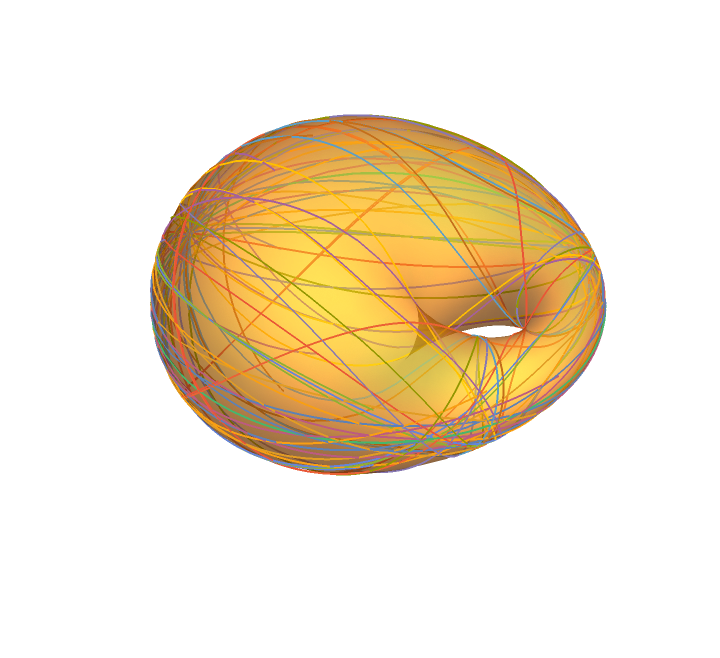
![sg = Flatten[
Table[NDSolve[
ResourceFunction["Geodesic"][
ResourceFunction["Cyclide"][8, 3, 5, {u, v}], {u, v}, t, {\[Pi], \[Pi]}, \[Theta]], {u, v}, {t, 0, 4 \[Pi]}], {\[Theta], 2 \[Pi]/30, 2 \[Pi], 2 \[Pi]/30}], 1];](https://www.wolframcloud.com/obj/resourcesystem/images/738/738c31bb-a402-448f-9fe1-8e66c2b28d5f/355755687a873e3f.png)
![Show[ParametricPlot3D[
Evaluate[ResourceFunction["Cyclide"][8, 3, 5, {u, v}]], {u, 0, 2 \[Pi]}, {v, 0, 2 \[Pi]}, PlotStyle -> Opacity[.5], Mesh -> False,
Boxed -> False, Axes -> False], ParametricPlot3D[
Evaluate[
ResourceFunction["Cyclide"][8, 3, 5][u[t], v[t]] /. sg], {t, 0, 2 \[Pi]}]]](https://www.wolframcloud.com/obj/resourcesystem/images/738/738c31bb-a402-448f-9fe1-8e66c2b28d5f/642adf185250ce6f.png)