Basic Examples (2)
Define a hyperbolic paraboloid:
The focal sets of the hyperbolic paraboloid are given by:
Plot an hyperbolic paraboloid (yellow) and its focal sets (blue and green):
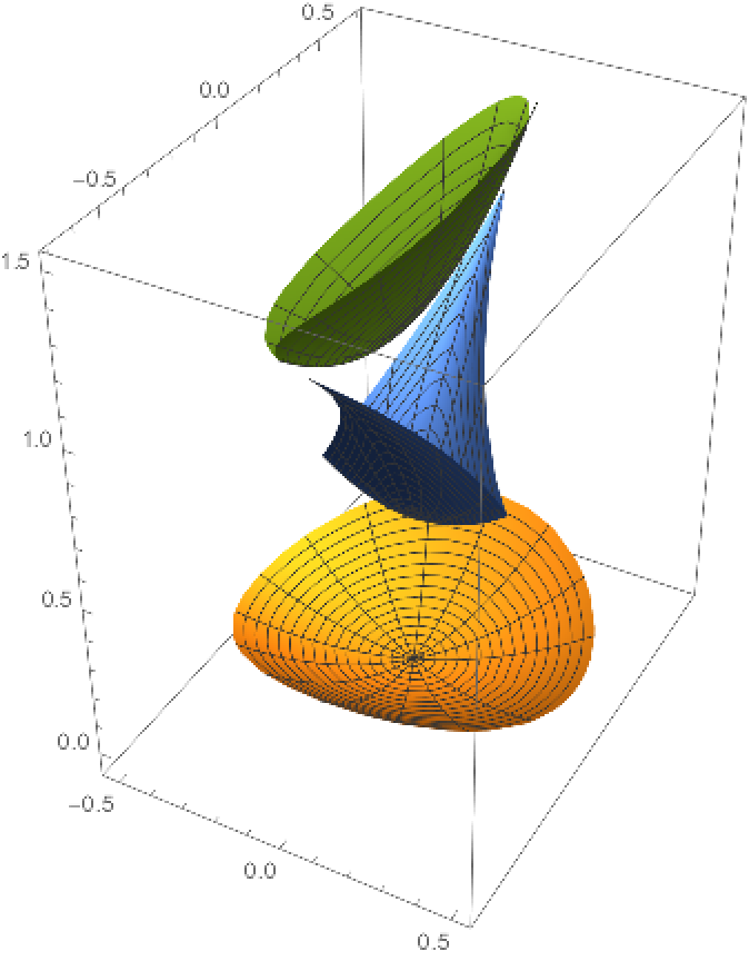
Define an elliptic paraboloid:
The focal sets of an elliptic paraboloid are given by:
Plot an elliptic paraboloid (yellow) and its focal sets (blue and green):
Scope (4)
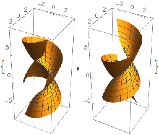
A circular helicoid:
Here are the two focal sets of the helicoid:
Plot the focal sets:
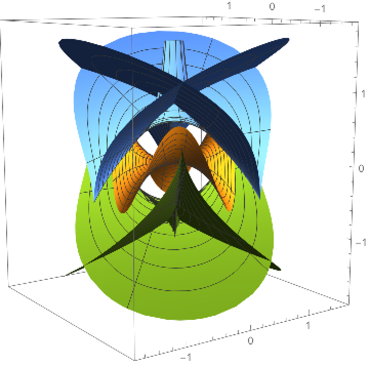
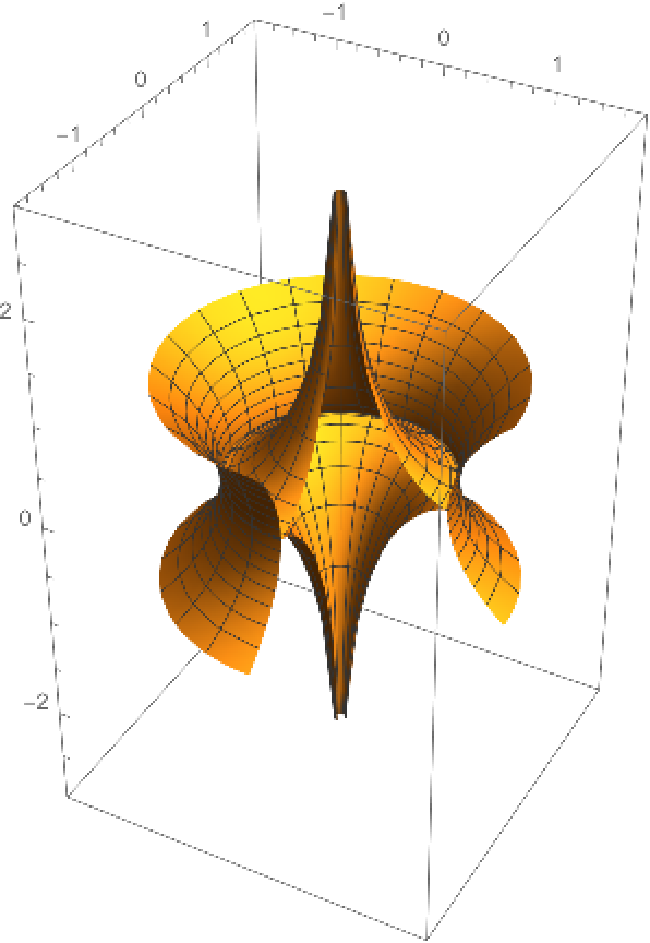
Compute the focal sets of a monkey saddle:
Plot of the focal sets of the monkey saddle:
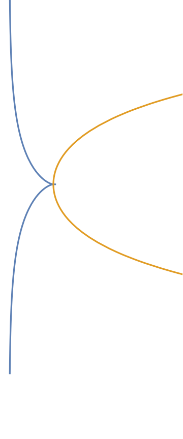
It will be shown in the next example that one of the focal sets of a surface of revolution generated by a plane curve c is the surface of revolution generated by the evolute of c. First define a tractrix:
Here is its evolute, as returned by the resource function EvoluteCurve:
The evolute of a tractrix is a catenary:
Define a catenoid, i.e. the surface of revolution of a catenary:
Define a surface of revolution:
Compute its focal set for the first curvature:
Plot the pseudosphere and the catenoid (the surface of revolution of a catenary) focal sets:
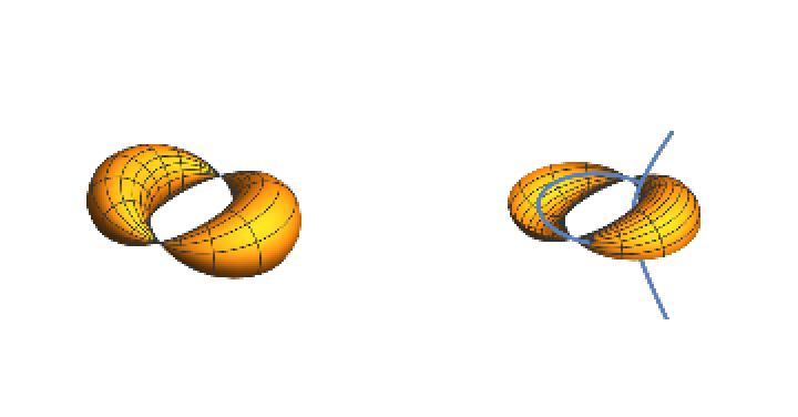
Define an elliptic‐hyperbolic cyclide:
Compute its focal sets:
Define a function to generate a cyclide together with its focal curves:
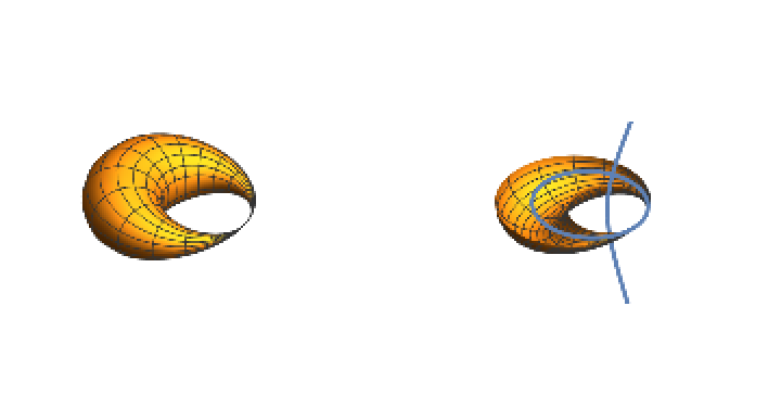
The ring cyclide with its focal curves:
The horn cyclide with its focal curves:
The spindle cyclide with its focal curves:

![Module[{f}, f[0] = hp; f[i_] := fshp[[i]]; ParametricPlot3D[
Evaluate[Table[f[i], {i, 0, 2}]], {u, -1, 1}, {v, -1, 1}]]](https://www.wolframcloud.com/obj/resourcesystem/images/7e0/7e0ba845-8cac-4a29-a957-4f0d08603956/6fd0ccf286c1f49a.png)


![Module[{f}, f[0] = ep; f[i_] := fsep[[i]]; ParametricPlot3D[
Evaluate[
Table[f[i] /. {u -> r Cos[\[Theta]], v -> r Sin[\[Theta]]}, {i, 0, 2}]], {r, 0, .5}, {\[Theta], 0, 2 \[Pi]}]]](https://www.wolframcloud.com/obj/resourcesystem/images/7e0/7e0ba845-8cac-4a29-a957-4f0d08603956/0bd1cf303e3a2461.png)

![ResourceFunction["FocalSet"][#, Entity["Surface", "MonkeySaddle"]["ParametricEquations"][1][u, v], {u, v}] & /@ {1, 2} // PowerExpand // FullSimplify](https://www.wolframcloud.com/obj/resourcesystem/images/7e0/7e0ba845-8cac-4a29-a957-4f0d08603956/00bd19ede396d66f.png)

![Module[{f}, f[0][u, v] = Entity["Surface", "MonkeySaddle"]["ParametricEquations"][1][u, v]; f[i_][u_, v_] := ResourceFunction["FocalSet"][i, f[0][u, v], {u, v}];
ParametricPlot3D[
Evaluate[
Table[f[i][u, v], {i, 0, 2}] /. {u -> r Cos[\[Theta]], v -> r Sin[\[Theta]]}], {r, 0.1, .85}, {\[Theta], 0, 2 \[Pi]}, PlotPoints -> {50, 30}, MaxRecursion -> 5, ViewPoint -> {-1.9, -2.73, 0.6}]]](https://www.wolframcloud.com/obj/resourcesystem/images/7e0/7e0ba845-8cac-4a29-a957-4f0d08603956/0cb323e45b7cdfd1.png)
![\[Alpha] = tractrix[1, t];
\[Epsilon] = ResourceFunction["EvoluteCurve"][\[Alpha], t];
ParametricPlot[{\[Alpha], \[Epsilon]}, {t, 0.01, \[Pi]}, Axes -> None]](https://www.wolframcloud.com/obj/resourcesystem/images/7e0/7e0ba845-8cac-4a29-a957-4f0d08603956/2932794872714713.png)
![pr = 1.6;
z[1] = ParametricPlot3D[
Evaluate[pseudosphere[1][u, v]], {u, 0, (3 \[Pi])/
2}, {v, .05, \[Pi] - .05}];
z[2] = ParametricPlot3D[
Evaluate[ca], {u, 0, (3 \[Pi])/2}, {v, .7, \[Pi] - .7}];
Show[Array[z, 2], PlotRange -> {{-pr, pr}, {-pr, pr}, Automatic}]](https://www.wolframcloud.com/obj/resourcesystem/images/7e0/7e0ba845-8cac-4a29-a957-4f0d08603956/1890615d3e696ca2.png)
![ellhypcyclide[a_, c_, k_][u_, v_] :=
Module[{A, B, s}, A = k - c Cos[u]; B = a - k Cos[v]; s = Sqrt[a^2 - c^2]; {c A + a Cos[u] B, s B Sin[u], s A Sin[v]}/(
a - c Cos[u] Cos[v])]](https://www.wolframcloud.com/obj/resourcesystem/images/7e0/7e0ba845-8cac-4a29-a957-4f0d08603956/7ccf41be89487ff8.png)
![cycgen[a_, c_, k_, rau_, rav_, opts___] :=
Module[{x, z, \[Alpha], \[Beta]}, x = ellhypcyclide[a, c, k]; z[1] = ParametricPlot3D[x[u, v], rau, rav, opts, Boxed -> False, Axes -> False]; \[Alpha][t_] := {a Cos[t], Sqrt[a^2 - c^2] Sin[t],
0}; \[Beta][t_] := {c Sec[t], 0, Sqrt[a^2 - c^2] Tan[t]}; z[2] = ParametricPlot3D[\[Alpha][t], {t, -\[Pi], \[Pi]}]; z[3] = ParametricPlot3D[\[Beta][t], {t, -.499 \[Pi], .499 \[Pi]}]; Show[Array[z, 3], PlotRange -> {{-a - c - k, a + c + k}, {-a - c - k, a + c + k}, {-a - c - k, a + c + k}}]]](https://www.wolframcloud.com/obj/resourcesystem/images/7e0/7e0ba845-8cac-4a29-a957-4f0d08603956/2fe6dfdb6edf93b3.png)
![x = ellhypcyclide[12, 3, 4.5];
z[1] = ParametricPlot3D[
Evaluate[x[u, v]], {u, 0, 2 \[Pi]}, {v, 0, 2 \[Pi]}, Boxed -> False, Axes -> False, PlotRange -> 19.5];
z[2] = cycgen[12, 3, 4.5, {u, 0, 2 \[Pi]}, {v, -\[Pi], 0}];
GraphicsGrid[{Array[z, 2]}]](https://www.wolframcloud.com/obj/resourcesystem/images/7e0/7e0ba845-8cac-4a29-a957-4f0d08603956/11f4ba38adfaa36e.png)

![x = ellhypcyclide[8, 4, 0];
z[1] = ParametricPlot3D[
Evaluate[x[u, v]], {u, 0, 2 \[Pi]}, {v, 0, 2 \[Pi]}, Boxed -> False, Axes -> False, PlotRange -> 12];
z[2] = cycgen[8, 4, 0, {u, 0, 2 \[Pi]}, {v, -\[Pi], 0}];
GraphicsGrid[{Array[z, 2]}]](https://www.wolframcloud.com/obj/resourcesystem/images/7e0/7e0ba845-8cac-4a29-a957-4f0d08603956/480865282198e9f7.png)
![Module[{x, z},
x = ellhypcyclide[12, 4, 4];
z[1] = ParametricPlot3D[x[u, v] // Evaluate,
{u, 0, 2 \[Pi]}, {v, 0, 2 \[Pi]}, Boxed -> False, Axes -> False, PlotRange -> 20];
z[2] = cycgen[12, 4, 4, {u, 0, 2 \[Pi]}, {v, -\[Pi], 0}]; GraphicsGrid[{Array[z, 2]}]
]](https://www.wolframcloud.com/obj/resourcesystem/images/7e0/7e0ba845-8cac-4a29-a957-4f0d08603956/1c663a63ea06f51c.png)