Basic Examples (7)
A sphere:
Equations for geodesics on a sphere:
A set of numerical solutions of equations for geodesics of a sphere:
Evaluate the geodesic at a definite point:
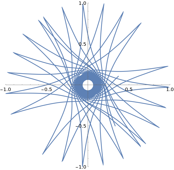
Plot solutions in a plane:
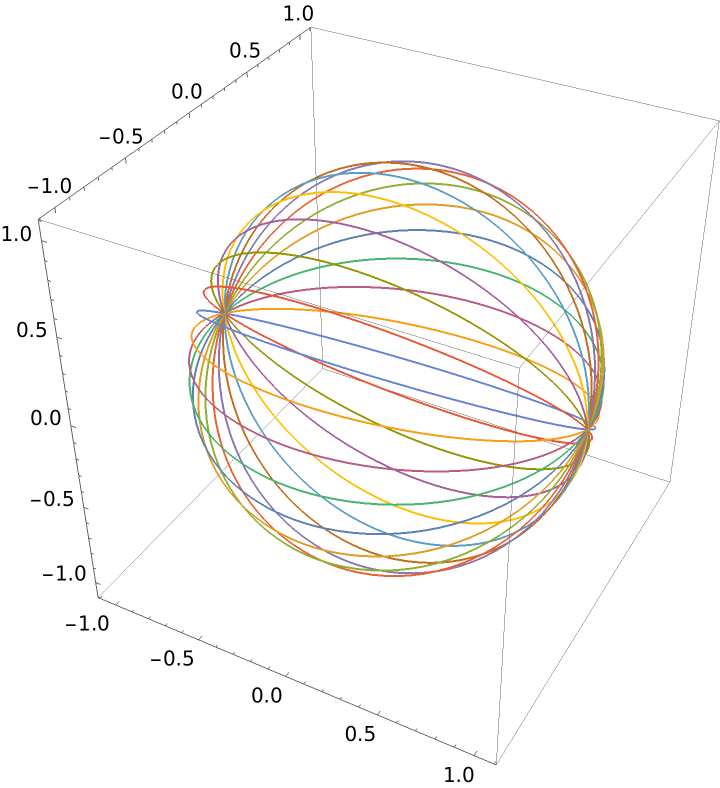
Plot geodesics on a sphere:
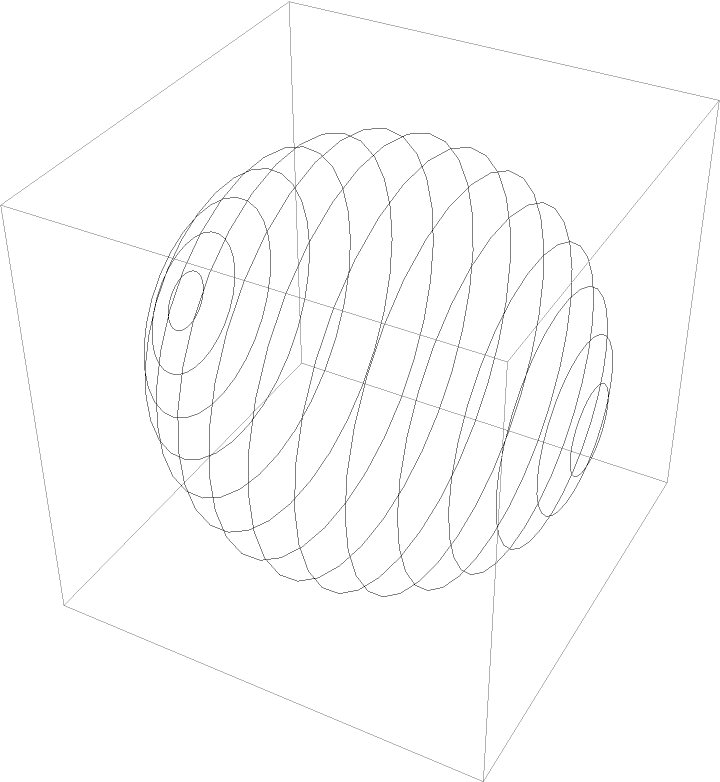
Plot the geodesic circles (locus surface points located at a given geodesic radius):
Scope (3)
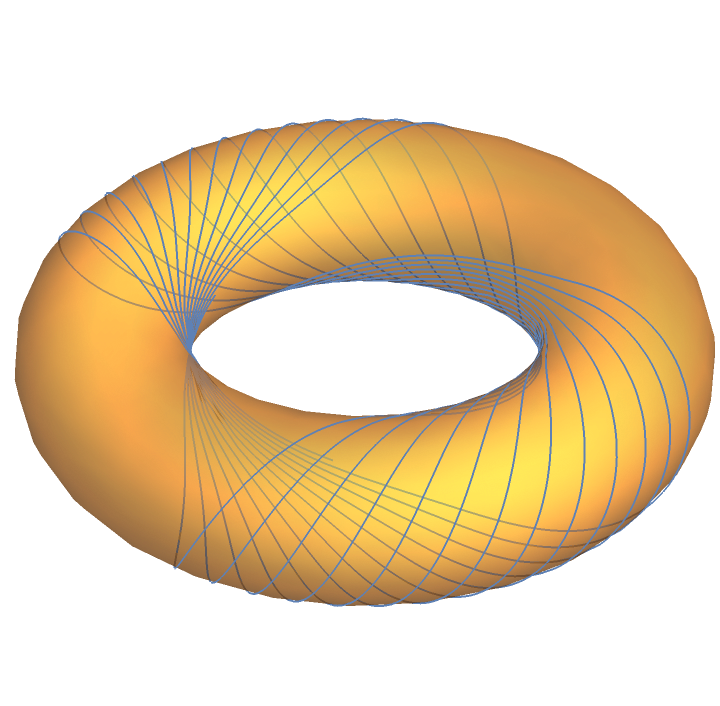
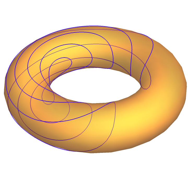
A torus:
The equations for geodesics:
Solve a geodesic for large t:
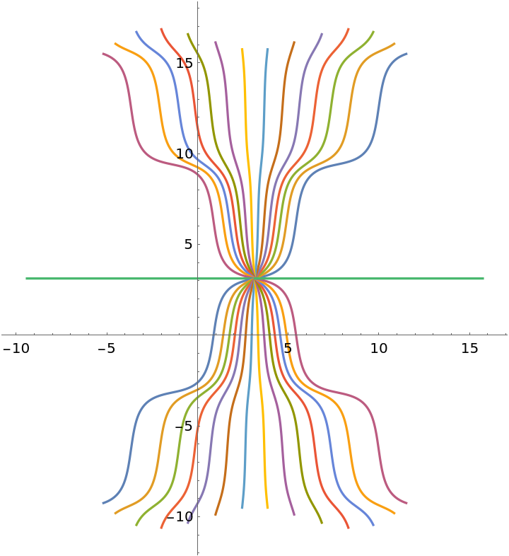
Solve for geodesics:
Plot solutions in a plane:
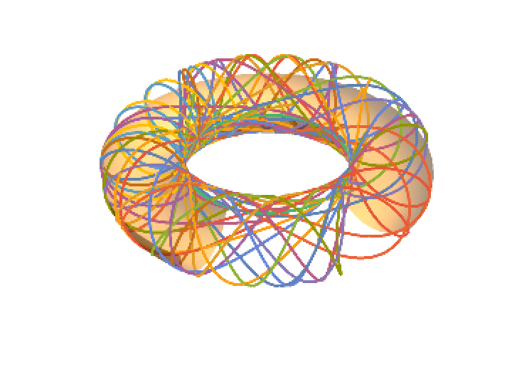
Solve for a set of geodesics:
Plot the geodesic circles:
Plot the geodesic circles over the torus:
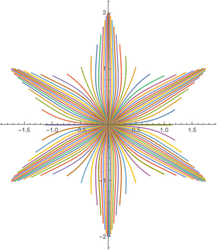
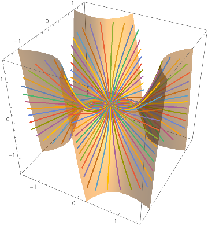
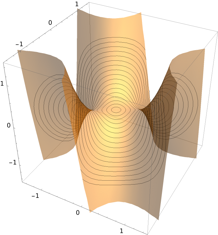
Define a monkey saddle:
Get the equations for geodesics:
Solve the equations for geodesics:
Plot solutions for geodesics:
Plot the geodesics over the surface:
Plot the geodesic circles:
Plot the geodesics circles over the surface:
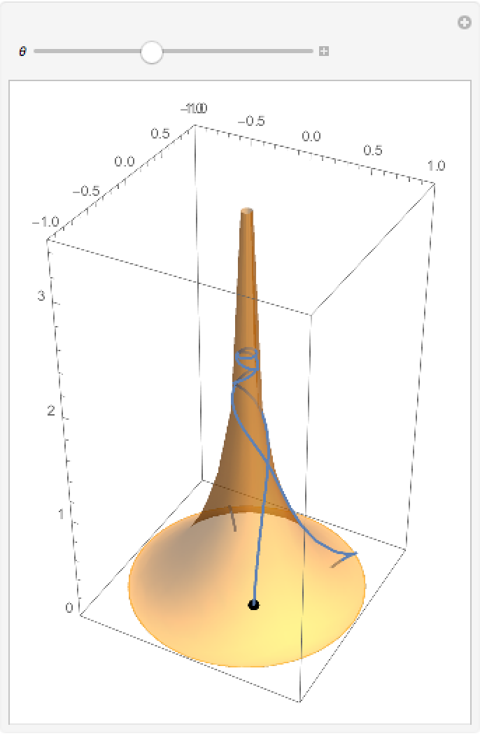
A pseudosphere:
The geodesic equations:
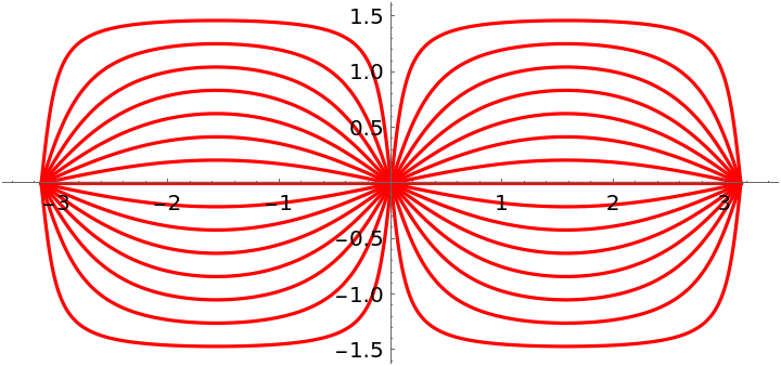
Plot the geodesic equations in 3D varying θ:
A top view of a solution:
![Show[ParametricPlot3D[
Evaluate[
torus[3, 1, 1][u[t], v[t]] /. NDSolve[ResourceFunction["Geodesic"][torus[3, 1, 1][u, v], {u, v},
t, {\[Pi], \[Pi]}, .5], {u, v}, {t, 0, 150}]], {t, 0, 150}, Boxed -> False, Axes -> False], ParametricPlot3D[
Evaluate[torus[3, 1, 1][u, v]], {u, 0, 2 \[Pi]}, {v, 0, 2 \[Pi]}, PlotStyle -> Opacity[.5], Mesh -> False]]](https://www.wolframcloud.com/obj/resourcesystem/images/88b/88bd3b54-bddf-4739-bc1b-d55b8a14d028/1945f9dad741b213.png)
![sg = Flatten[
Table[NDSolve[
ResourceFunction["Geodesic"][torus[3, 1, 1][u, v], {u, v}, t, {\[Pi], \[Pi]}, \[Theta]], {u, v}, {t, 0, 4 \[Pi]}], {\[Theta], 2 \[Pi]/30, 2 \[Pi], 2 \[Pi]/30}], 1];](https://www.wolframcloud.com/obj/resourcesystem/images/88b/88bd3b54-bddf-4739-bc1b-d55b8a14d028/05da3c04856a59df.png)
![Show[ParametricPlot3D[
Evaluate[torus[3, 1, 1][u, v]], {u, 0, 3 \[Pi]/2}, {v, \[Pi], 2 \[Pi]}, PlotStyle -> Opacity[.5], Mesh -> False, Boxed -> False, Axes -> False], ParametricPlot3D[
Evaluate[torus[3, 1, 1][u[t], v[t]] /. sg], {t, 0, 4 \[Pi]}]]](https://www.wolframcloud.com/obj/resourcesystem/images/88b/88bd3b54-bddf-4739-bc1b-d55b8a14d028/7de40e680f17f5a7.png)
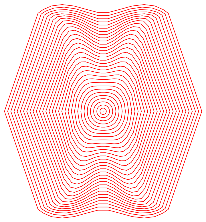
![sg = Flatten[
Table[NDSolve[
ResourceFunction["Geodesic"][torus[3, 1, 1][u, v], {u, v}, t, {\[Pi], \[Pi]}, \[Theta]], {u, v}, {t, 0, 2.5}], {\[Theta], 2 \[Pi]/200, 2 \[Pi], 2 \[Pi]/200}], 1];](https://www.wolframcloud.com/obj/resourcesystem/images/88b/88bd3b54-bddf-4739-bc1b-d55b8a14d028/20c10a77b8863a90.png)
![ta = Table[
Line[Append[#, First[#]] &[torus[3, 1, 1][u[t], v[t]] /. sg]], {t, 0, 2.5, .5}];
Show[Graphics3D[{Thickness[.005], Hue[.7], ta}], ParametricPlot3D[
Evaluate[torus[3, 1, 1][u, v]], {u, 0, 2 \[Pi]}, {v, 0, 2 \[Pi]}, PlotStyle -> Opacity[.5], Mesh -> False, Boxed -> False, Axes -> False], Boxed -> False]](https://www.wolframcloud.com/obj/resourcesystem/images/88b/88bd3b54-bddf-4739-bc1b-d55b8a14d028/49f91bd6b76c20a8.png)

![sd = With[{u0 = 0, v0 = 0, a = 0, n = 100, tf = 2}, Flatten[((NDSolve[#1, {u, v}, {t, 0, 2}]) &) /@ Table[ge, {\[Theta], (2 \[Pi])/n, 2 \[Pi], (2 \[Pi])/n}], 1]];](https://www.wolframcloud.com/obj/resourcesystem/images/88b/88bd3b54-bddf-4739-bc1b-d55b8a14d028/382f9148de3be9e0.png)
![Show[ParametricPlot3D[Evaluate[ms], {u, -2, 2}, {v, -\[Pi], \[Pi]}, PlotRange -> 1.5, PlotStyle -> Opacity[.5], Mesh -> False], ParametricPlot3D[
Evaluate[ms /. {u -> u[t], v -> v[t]} /. sd], {t, 0, 2}]]](https://www.wolframcloud.com/obj/resourcesystem/images/88b/88bd3b54-bddf-4739-bc1b-d55b8a14d028/582803bce681c18f.png)

![Show[ParametricPlot3D[Evaluate[ms], {u, -2, 2}, {v, -\[Pi], \[Pi]}, PlotRange -> 1.5, PlotStyle -> Opacity[.5], Mesh -> False], Graphics3D[
Table[Line[
Append[ms /. {u -> u[t], v -> v[t]} /. sd, ms /. {u -> u[t], v -> v[t]} /. sd[[1]]]], {t, 0, 1.7, .1}]]]](https://www.wolframcloud.com/obj/resourcesystem/images/88b/88bd3b54-bddf-4739-bc1b-d55b8a14d028/45188a4d805be75b.png)
![plot = Show[
ParametricPlot3D[.99 pseudosphere[1][u, v], {u, 0, 2 \[Pi]}, {v, 0, \[Pi] - .01}, Mesh -> None, PlotStyle -> Opacity[.5]], Graphics3D[{PointSize[.03], Point[pseudosphere[1] @@ P]}]];](https://www.wolframcloud.com/obj/resourcesystem/images/88b/88bd3b54-bddf-4739-bc1b-d55b8a14d028/1351909150024d7d.png)
![Manipulate[
Show[ParametricPlot3D[
Evaluate[
pseudosphere[1][u[t], v[t]] /. NDSolve[ResourceFunction["Geodesic"][
pseudosphere[1][u, v], {u, v}, t, P, \[Theta]], {u, v}, {t, 0, 10}]], {t, 0, 10}, PlotRange -> {{-1, 1}, {-1, 1}, {0, 3.5`}}],
plot], {{\[Theta], 1.3}, 0, \[Pi]}]](https://www.wolframcloud.com/obj/resourcesystem/images/88b/88bd3b54-bddf-4739-bc1b-d55b8a14d028/7733f6a1c66b173b.png)
![Module[{\[Theta] = 1.3`}, ParametricPlot[
Evaluate[
Most[First[
pseudosphere[1][u[t], v[t]] /. NDSolve[ResourceFunction["Geodesic"][
pseudosphere[1][u, v], {u, v}, t, P, \[Theta]], {u, v}, {t, 0,
120}]]]], {t, 0, 120}, PlotRange -> 1]]](https://www.wolframcloud.com/obj/resourcesystem/images/88b/88bd3b54-bddf-4739-bc1b-d55b8a14d028/74e574910b2dfaad.png)