Wolfram Function Repository
Instant-use add-on functions for the Wolfram Language
Function Repository Resource:
Compute the involute of a curve
ResourceFunction["InvoluteCurve"][c,t] computes the involute of a curve c with parameter t. | |
ResourceFunction["InvoluteCurve"][c,{t,tf}] computes the involute by switching to numerical integration from 0 to tf. |
Compute the involute of a circle:
| In[1]:= |
![\[Alpha] = Entity["PlaneCurve", "Circle"]["ParametricEquations"][1][t];
invc = ResourceFunction["InvoluteCurve"][\[Alpha], t] // Simplify](https://www.wolframcloud.com/obj/resourcesystem/images/715/715c88ab-0c1d-442e-b07d-0eda53d73190/3baf405c846de9a3.png)
|
| Out[1]= |
|
Plot the circle involute and tangent lines along the circle:
| In[2]:= |
![z[k_] := Line[{\[Alpha], invc} /. t -> (\[Pi] k)/7]
ParametricPlot[Evaluate[{\[Alpha], invc}], {t, 0, 2 \[Pi]}, Epilog -> Array[z, 14], Axes -> False]](https://www.wolframcloud.com/obj/resourcesystem/images/715/715c88ab-0c1d-442e-b07d-0eda53d73190/316d40964c50bcf2.png)
|
| Out[2]= |
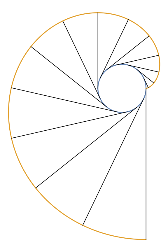
|
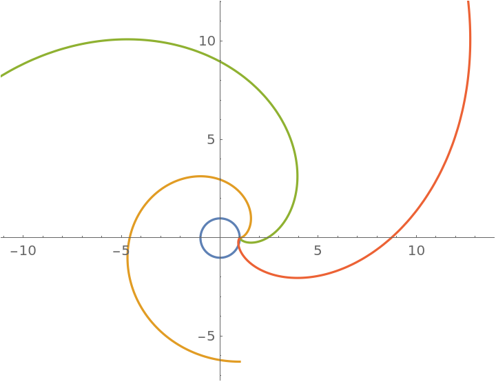
Start the involute at π/2:
| In[3]:= |
![p = 15;
ParametricPlot[
Evaluate[{\[Alpha], invc, ResourceFunction["InvoluteCurve"][\[Alpha] /. t -> t + \[Pi]/2, t]}], {t, 0, p}, PlotRange -> {{-p, p}, {-p, p}}]](https://www.wolframcloud.com/obj/resourcesystem/images/715/715c88ab-0c1d-442e-b07d-0eda53d73190/7471b1a3bd3417ee.png)
|
| Out[3]= |
|
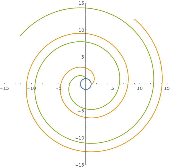
Nested involutes of the circle:
| In[4]:= |
|
| Out[4]= |
|
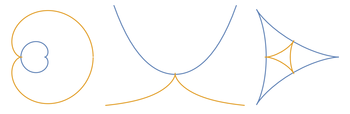
Here are some involute plots for several named curves:
| In[5]:= |
![InvoluteCurvePlot[c_, {t_, t0_, tf_}, opts___] := ParametricPlot[
Evaluate[{c, ResourceFunction["InvoluteCurve"][c, t]}], {t, t0, tf}, opts, Axes -> False];
GraphicsRow[{InvoluteCurvePlot[
Entity["PlaneCurve", "Cardioid"]["ParametricEquations"][1][t], {t, 0.01, 2 \[Pi] - .01}], InvoluteCurvePlot[
Entity["PlaneCurve", "Catenary"]["ParametricEquations"][1][
t], {t, -3, 3}, PlotRange -> {{-2, 2}, {0, 3}}], InvoluteCurvePlot[
Entity["PlaneCurve", "Deltoid"]["ParametricEquations"][1][t], {t, 0.01, 2 \[Pi] - .01}]}]](https://www.wolframcloud.com/obj/resourcesystem/images/715/715c88ab-0c1d-442e-b07d-0eda53d73190/6d1d763df690fbfa.png)
|
| Out[5]= |
|
The evolute of a curve's involute is the curve itself:
| In[6]:= |
|
| Out[6]= |
|
The eight curve:
| In[7]:= |
|
The involute curve:
| In[8]:= |
|
| Out[8]= |
|
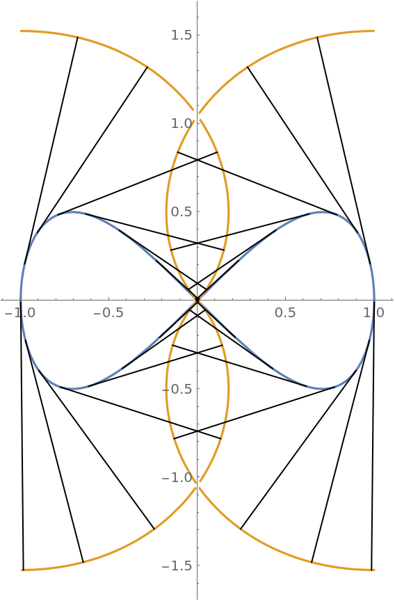
The involute curve using the expression shown above gives the same result four times:
| In[9]:= |
![z1[k_] := Line[{eight[t], ResourceFunction["InvoluteCurve"][eight[t], t]} /. t -> (\[Pi] k)/14 + .01]
ParametricPlot[Evaluate[{eight[t], f}], {t, 0.01, 2 \[Pi] - .01}, Epilog -> Array[z1, 28]]](https://www.wolframcloud.com/obj/resourcesystem/images/715/715c88ab-0c1d-442e-b07d-0eda53d73190/60fb09e28db373dc.png)
|
| Out[9]= |
|
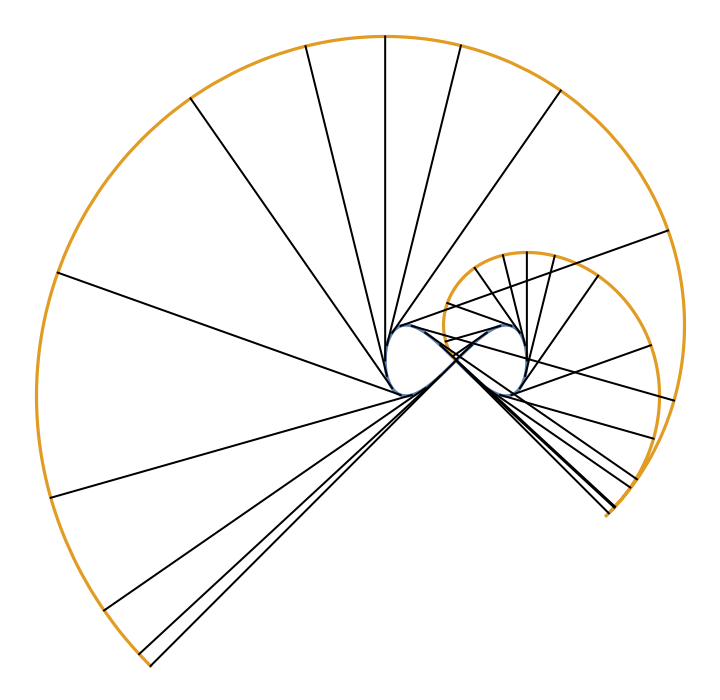
Using numerical integration gives the correct result:
| In[10]:= |
![z[k_] := Line[{eight[tf], ResourceFunction["InvoluteCurve"][
eight[tf], {tf, (\[Pi] k)/14}]} /. tf -> (\[Pi] k)/14]
ParametricPlot[{eight[tf], ResourceFunction["InvoluteCurve"][eight[t], {t, tf}] /. t -> tf}, {tf, 0.01, 2 \[Pi]}, Epilog -> Array[z, 28], Axes -> False]](https://www.wolframcloud.com/obj/resourcesystem/images/715/715c88ab-0c1d-442e-b07d-0eda53d73190/555c9fa4e45758b1.png)
|
| Out[10]= |
|
This work is licensed under a Creative Commons Attribution 4.0 International License