Wolfram Function Repository
Instant-use add-on functions for the Wolfram Language
Function Repository Resource:
Compute a rolling curve
ResourceFunction["RollingCurve"][c,r,h,t0,t] gives the parametrized curve traced out by a point P attached to a circle of radius r rolling along a plane curve c parametrized by variable t. The distance from P to the center of the rolling circle is h, and t0 is the point of the curve at which the circle starts rolling. | |
ResourceFunction["RollingCurve"][c,r,t0,t] takes the distance from the tracing point to the center of the rolling circle to be Abs[r]. |
Define the parametric equations for an ellipse:
| In[1]:= |
|
| Out[1]= |
|
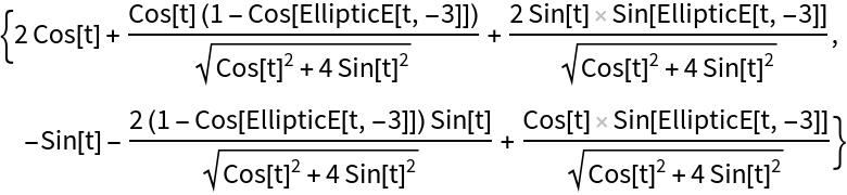
Compute the rolling curve of the ellipse:
| In[2]:= |
|
| Out[2]= |
|
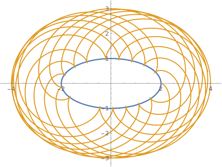
Plot the rolling curve:
| In[3]:= |
|
| Out[3]= |
|
Parametric equations for a circle:
| In[4]:= |
|
The epitrochoid is the rolling curve of a circle if the rolling circle is outside the original circle:
| In[5]:= |
|
| Out[5]= |
|
The epicycloid is obtained if ![]() :
:
| In[6]:= |
|
| Out[6]= |
|
An equivalent way to get the epicycloid:
| In[7]:= |
|
| Out[7]= |
|
Define the parametric equations of a parabola:
| In[8]:= |
|
| Out[8]= |
|
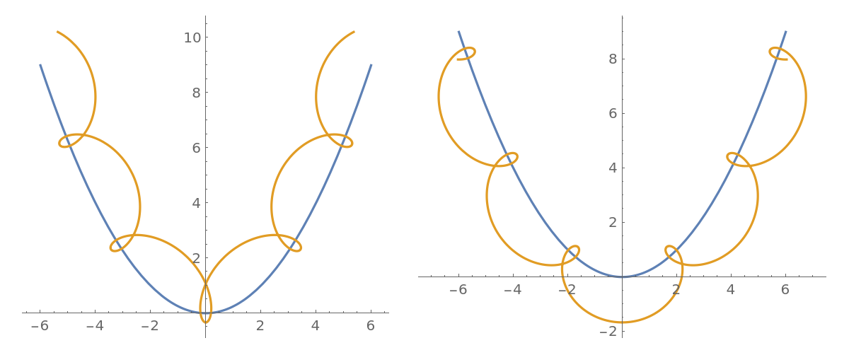
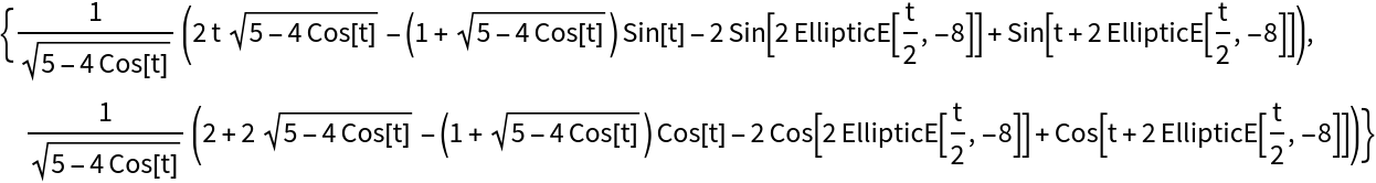
Define the rolling curve of the parabola:
| In[9]:= |
|
| Out[9]= |

|
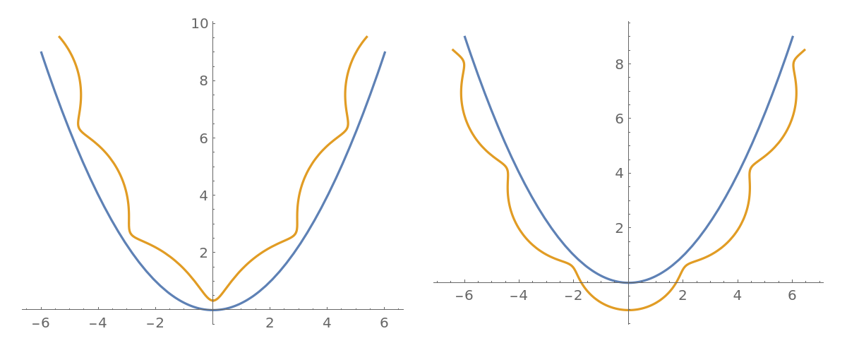
When ![]() (the curtate case), the rolling curve is smooth:
(the curtate case), the rolling curve is smooth:
| In[10]:= |
|
| Out[10]= |
|
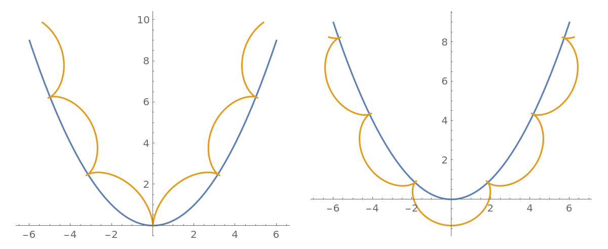
When ![]() (the cycloidal case), the rolling curve has cusps:
(the cycloidal case), the rolling curve has cusps:
| In[11]:= |
|
| Out[11]= |
|
When ![]() (the prolate case), the rolling curve has self-intersection points:
(the prolate case), the rolling curve has self-intersection points:
| In[12]:= |
|
| Out[12]= |
|
Define the parametric equations of a trochoid:
| In[13]:= |
|
| Out[13]= |
|
Compute the parallel curve of the trochoid:
| In[14]:= |
|
| Out[14]= |
|
Compute the rolling curve of the trochoid:
| In[15]:= |
|
| Out[15]= |
|
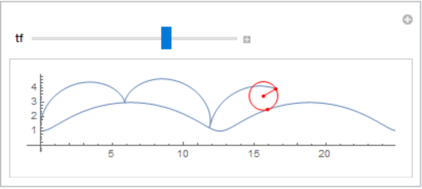
Create a Manipulate that rolls a circle along the curve:
| In[16]:= |
![Manipulate[
Show[ParametricPlot[Evaluate[rcc], {t, 0, tf}, Epilog -> {Directive[Red, PointSize[0.01]], Circle[par /. t -> tf],
Line[{par /. t -> tf, rcc /. t -> tf}], Point[{trochoid[2, 1][tf], par /. t -> tf, rcc /. t -> tf}]}, Axes -> True, PlotRange -> {{-0.96, 24.85}, {-.5, 4.98}}], ParametricPlot[Evaluate[trochoid[2, 1][t]], {t, 0, 4 \[Pi]}]], {{tf,
8.4}, .01, 4 \[Pi]}]](https://www.wolframcloud.com/obj/resourcesystem/images/9e0/9e0fd377-18df-4f09-b408-de9a63be7fb0/6b036f9f99da5073.png)
|
| Out[16]= |
|
This work is licensed under a Creative Commons Attribution 4.0 International License