Scope (7)
Start with a set of approximate real values:
Use the weight argument to find rational approximations with a small common denominator:
With a larger weight we obtain closer approximations:
With a sufficiently small weight we find integer approximations:
SimultaneousRationalize can work with rationals in the input:
Find rational approximations with a smaller common denominator:
The values in question are approximately commensurate, i.e. all are multiples of a common value. In this case the smallest element in the list:
Possible Issues (2)
Values that are small in magnitude compared to unity will often be approximated by zero:
Use a weight commensurate with the reciprocal of the smallest value to force the approximation to be nonzero:
Neat Examples (9)
Simultaneous rationalization can be used on light curve data to estimate the period of a variable star. We will take for our example Kepler project data for the Cepheid star 2308. The reference period at the OGLE web site is given as 5.7373087 days. Data and more can also be found at the Wolfram Demonstration "CepheidVariableStarLightCurve" by Jeffrey Bryant. This example is also found in the resource function IrregularPeriodogram.
Import the data from OGLE:
Separate into observation times and light intensities, and subtract the average from the set of values:
We extract candidate period multiples as follows. The idea is that "common" time differences for approximately equal values correspond to times that are separated by a multiple of the basic period. (1) Compute an ϵ for proximity (a small fraction of the range of values). (2) Find all time differences between pairs that have their respective values within this ϵ. (3) Separate time differences into bins according to whether they are in proximity. This step uses an input threshold for proximity, with default of 0.1. (4) Cull out those time differences that do not appear often. This step uses an input minimum for bin sizes, with default of 15. (5) Take means of each retained bin. These are the candidate approximations for multiples of periodicities.
Utility function to find candidate periodicity multiples:
Compute candidate periodicity multiples for Cepheid 2308:
Remove the smallest value since it is too small to be a period and is most likely an artifact of the average sampling time gap:
Use simultaneous Diophantine approximation to find integer ratios that approximate the period multiple ratios:
Divide the approximated period multiples by the approximated multipliers (the initial multiplier is assumed to be unity):
Take the average to get our period approximation:
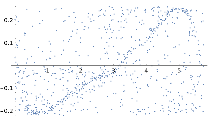
Fold the light curve by this estimated period:
The "fuzz" points are due to the estimate being off in the second decimal place, but still one can clearly discern the main wave pattern.
![data = {.003245, 5.831666666666677`, 22.96202080402009`, 40.0120210909091`, 45.92557465116284`};
ResourceFunction["SimultaneousRationalize"][data]](https://www.wolframcloud.com/obj/resourcesystem/images/621/62166eaf-367f-4059-8ded-f72616a13484/08104640a38f9cc9.png)
![cep2308Idata = Import[
"http://ogledb.astrouw.edu.pl/~ogle/CVS/data/I/08/OGLE-LMC-CEP-2308.dat"
, "Table"][[All, 1 ;; 2]];](https://www.wolframcloud.com/obj/resourcesystem/images/621/62166eaf-367f-4059-8ded-f72616a13484/5683000176c893e6.png)
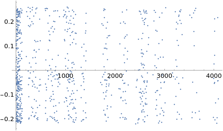
![{times2308, ovalues2308} = Transpose[cep2308Idata];
times2308 = times2308 - times2308[[1]];
mean2308 = Mean[ovalues2308];
values2308 = ovalues2308 - mean2308;
ListPlot[Transpose@{times2308, values2308}]](https://www.wolframcloud.com/obj/resourcesystem/images/621/62166eaf-367f-4059-8ded-f72616a13484/29bf0f8c8600186f.png)
![periodMultiples[vals_, times_, minrunlen_ : 15, frac_ : 300, thresh_ : .1] := Module[
{nfunc, eps, nbrs, nbrsSplit, xdiffs, splitdiffs},
nfunc = Nearest[vals -> Range[Length[vals]]];
eps = (Max[vals] - Min[vals])/frac;
nbrs = Table[nfunc[valj, {Infinity, eps}], {valj, vals}];
nbrsSplit = Map[{First[#], Rest[#]} &, nbrs];
xdiffs = Sort[Flatten[
Abs[Table[
times[[nbhdj[[1]]]] - times[[nbrjk]], {nbhdj, nbrsSplit}, {nbrjk, nbhdj[[2]]}]]]];
splitdiffs = Split[xdiffs, Abs[#2 - #1] < thresh &];
Map[Mean, Select[splitdiffs, Length[#] >= minrunlen &]]
]](https://www.wolframcloud.com/obj/resourcesystem/images/621/62166eaf-367f-4059-8ded-f72616a13484/790fa606de8f76d7.png)