Basic Examples (10)
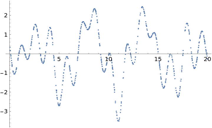
Take random times and corresponding values for the function f(t)=sin(t)+cos(3t)/2:
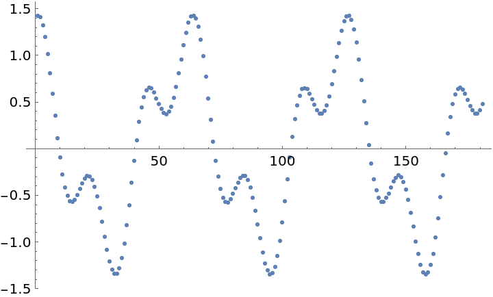
Subtract the mean of the data values and plot the resulting time series:
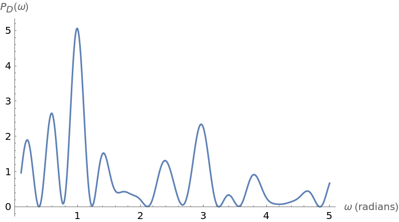
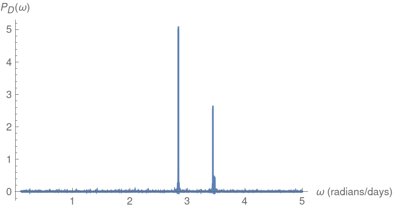
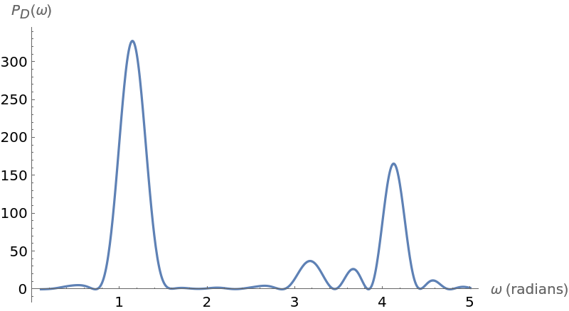
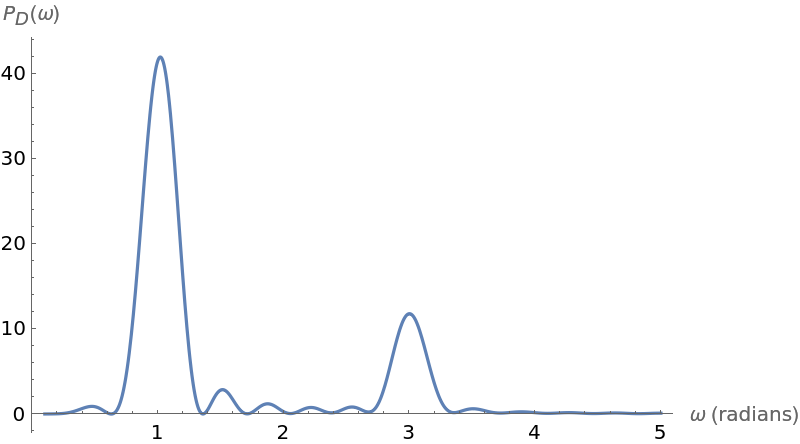
Plot the periodogram computed from this unevenly spaced set of measurements:
Compute the larger frequency (the location of the larger spike):
Compute the period from this frequency:
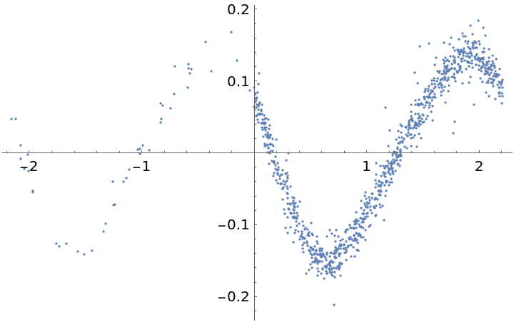
Plot the time series "folded" by this period (times are computed modulo the computed period) to see the approximately sinusoidal variation in the light curve:
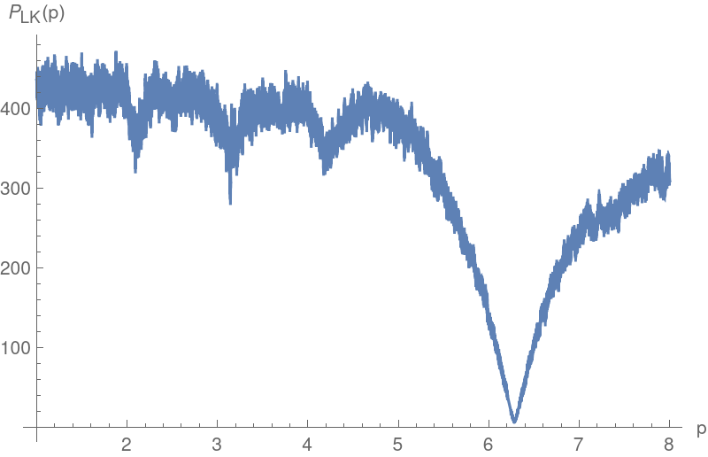
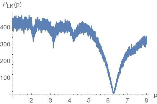
The string-length approach also shows this periodicity:
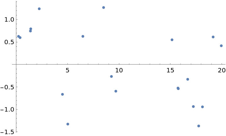
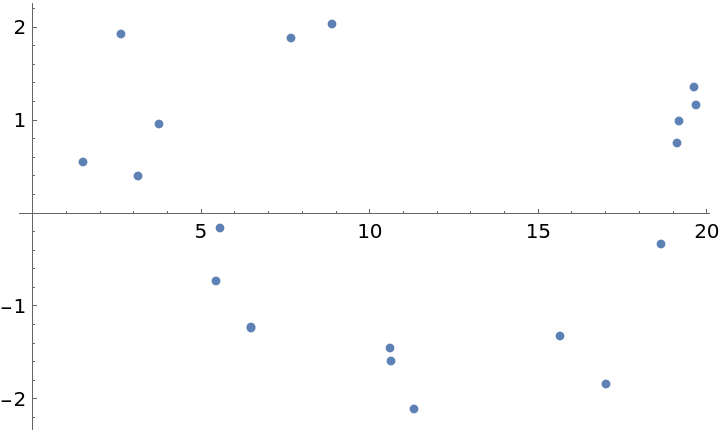
One can get a fairly good estimate of the frequencies present using far fewer samples, so long as they are irregularly spaced in time. Take 20 random points from the preceding original set:
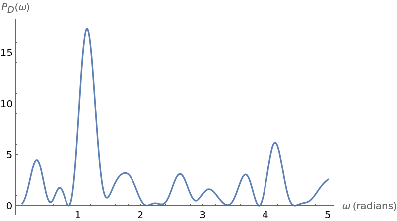
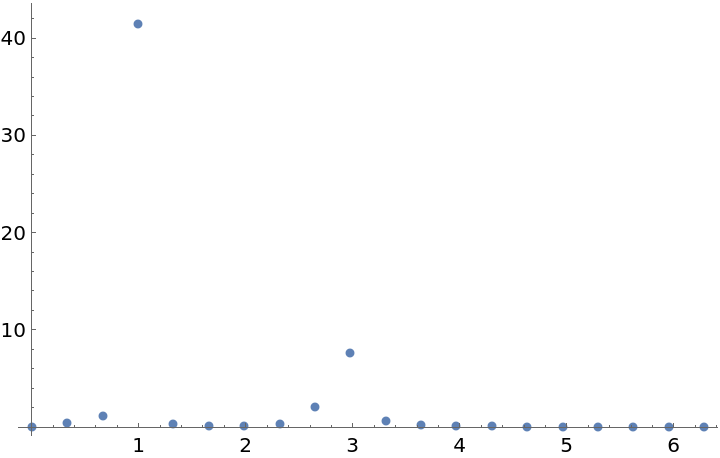
Plot the periodogram from this subset:
Estimate the period for the larger frequency:
Scope (2)
Use a light curve time series from the Wolfram Demonstration Cepheid Variable Star Light Curve Analysis:
Subtract the mean of the data values and plot the resulting time series:
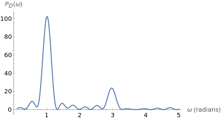
Plot the periodogram computed from this unevenly spaced set of measurements:
Compute the main frequency as the location of the larger spike:
Compute the period from this frequency:
Plot the time series "folded" by this period (times are computed modulo the computed period) to see the approximately sinusoidal variation in the light curve:
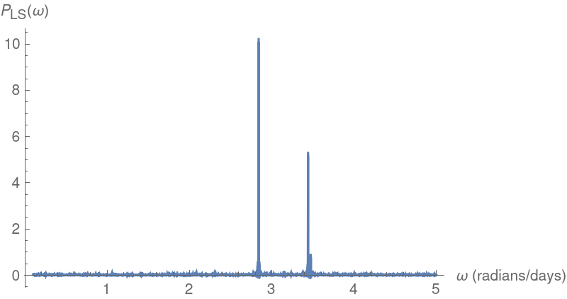
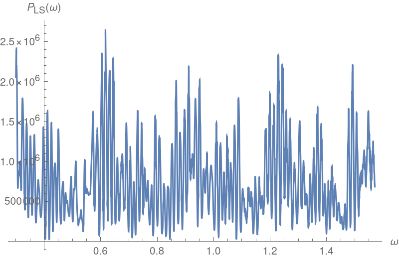
Plot the Lomb-Scargle periodogram for the same data:
The computed main frequency and period agree with the values from the Deeming periodogram:
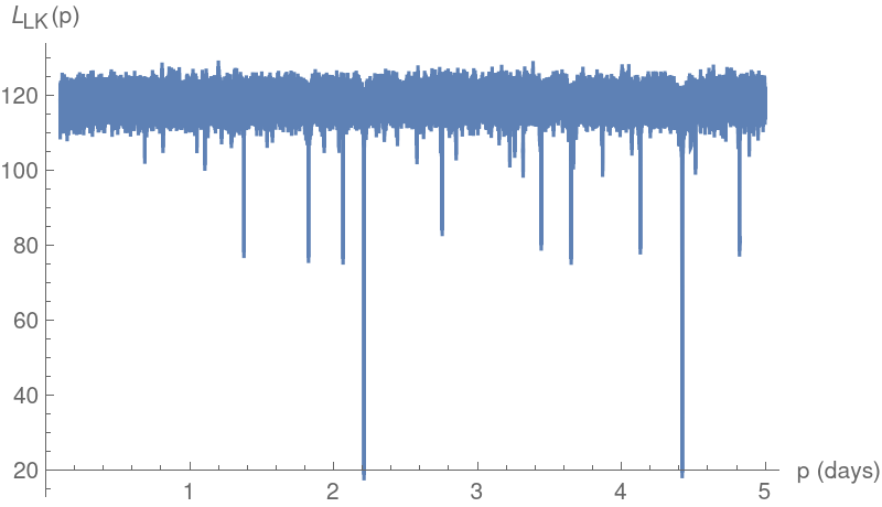
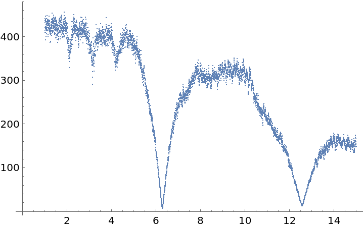
Plot the string-length values for the same data:
Compute the best estimate for the period based on the minimum value attained by the Lafler-Kinman computation for this data:
A periodogram can often detect multiple frequencies provided they are well separated, even if they are not commensurate (that is, there is no actual “period” for the data). Extract values from such a function with frequencies at 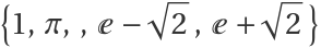 :
:
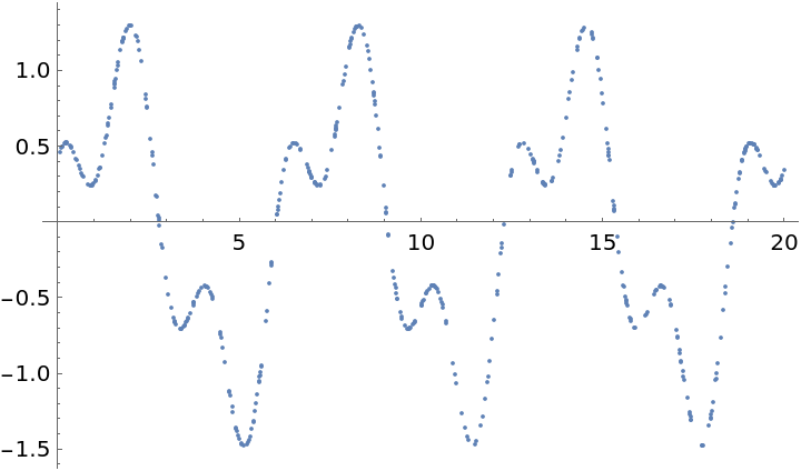
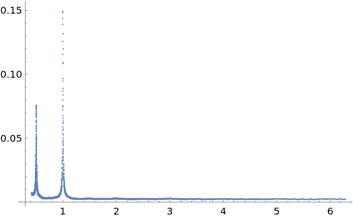
Plot the periodogram for this data:
There is one estimated frequency around midway between 1 and  :
:
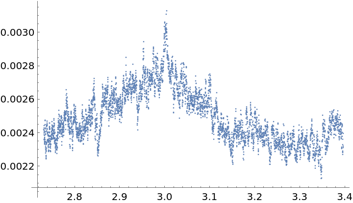
Another is approximately π:
A third is close to  :
:
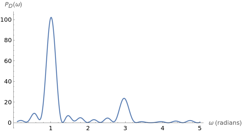
Rough estimates can be made with far fewer sampled values:
Peaks of the periodogram give estimates of the frequencies:
Properties & Relations (2)
When the data is equally spaced on the horizontal axis, the irregular periodogram is essentially the square of the Fourier transform. Modify a previous example to demonstrate this:
Subtract the mean of the data values and plot the resulting time series:
Plot the periodogram computed from this (evenly-) spaced set of measurements:
The square of the Fourier transform gives a similar result once frequencies are correctly rescaled on the horizontal axis:
In the Wolfram Language, this can also be computed using PeriodogramArray:
Yet another way to obtain these absolute values is with the Fourier transform of the set of values convolved with itself:
The Lafler-Kinman string-lengths-based measure can be made to more closely resemble an ordinary periodogram using reciprocals. Use a basic example:
Now again show the Lafler-Kinman plot using this data:
It is possible to go from time to frequency using the formula f=2π/t, and likewise go from small to large on the vertical axis by taking reciprocals:
Generate and plot a list of {foldtime,magnitude} pairs:
Now do the transformation and replot:
The main spike coincides with that of the Deeming periodogram. There is a small bump in the Deeming periodogram near frequency 3. For the Lafler-Kinman version, this corresponds to a fold time near 2.1:
Compute a lot of values in the vicinity of this folding time:
Applications (43)
Sunspot activity cycles (10)
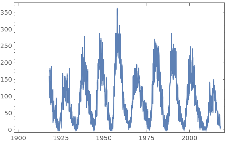
Sunspot activity follows an approximately 11-year cycle. Download a century of monthly averaged values from the Wolfram Data Repository:
Show the plot for this time series:
Obtain the times and mean-centered values:
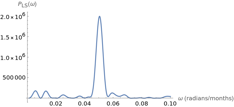
Plot the Deeming periodogram for this time series:
Compute the maximum frequency and the corresponding estimated period in months:
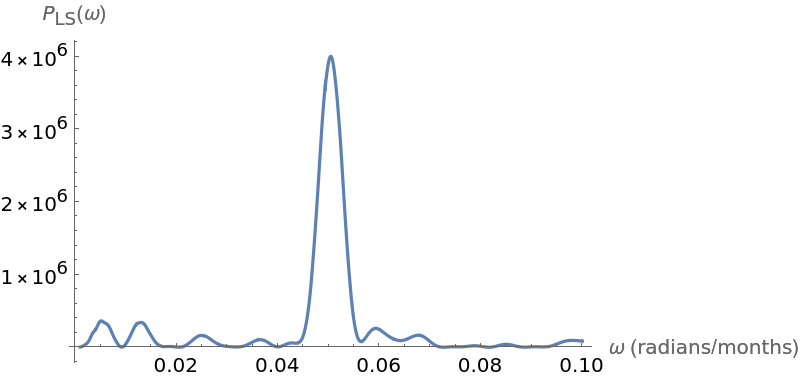
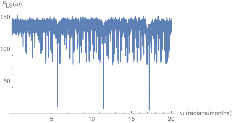
Plot the Lomb-Scargle periodogram for this time series:
Compute the maximum frequency and the corresponding estimated period in months:
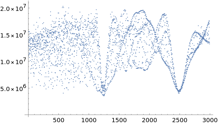
Plot a list of string lengths versus folding period for this time series:
Compute the estimated period from the low point position:
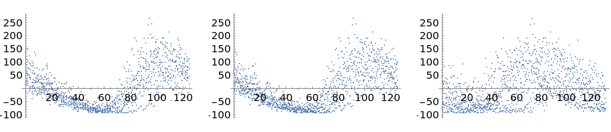
All three estimates are in the ballpark of 10.5 years. Plot the time series epoch-folded by the second and third period estimates, as well as by the conventional 11 years:
Another cepheid variable star analysis (6)
Download and process times and values of the light curve for the variable star known as cep2308:
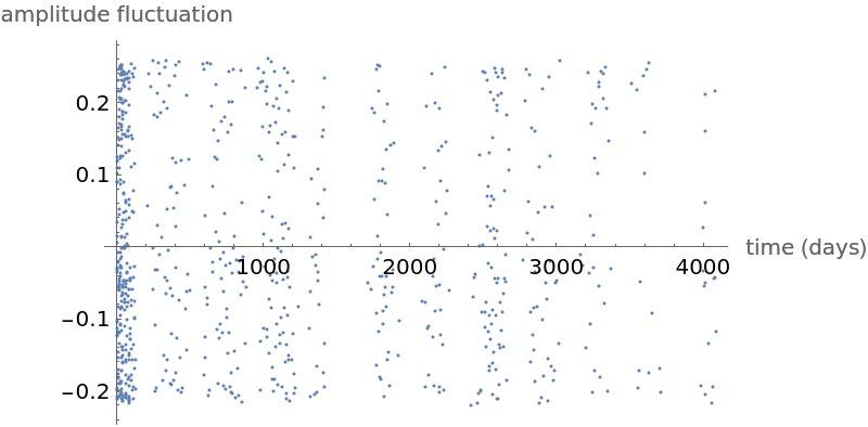
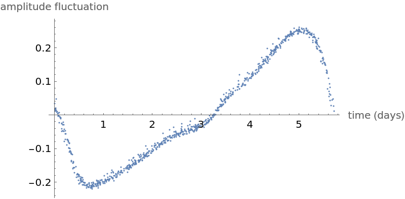
Show a plot of measured amplitudes over time:
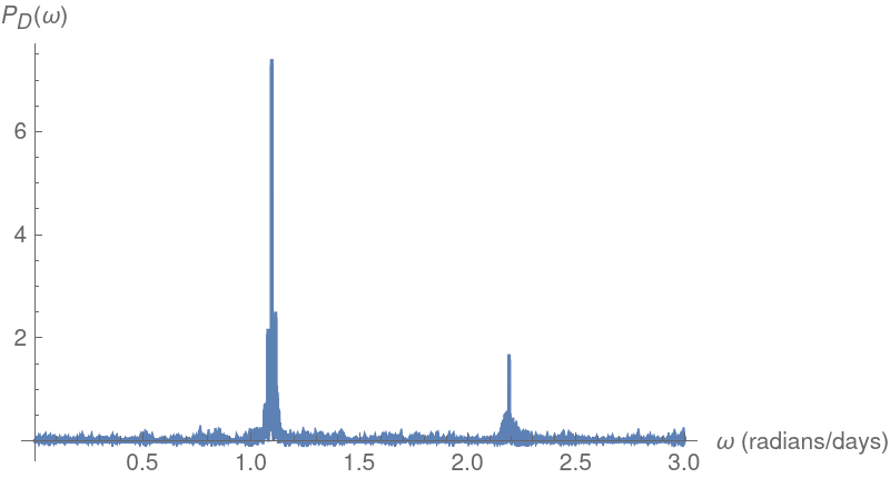
Plot the Deeming periodogram and compute the corresponding estimated period:
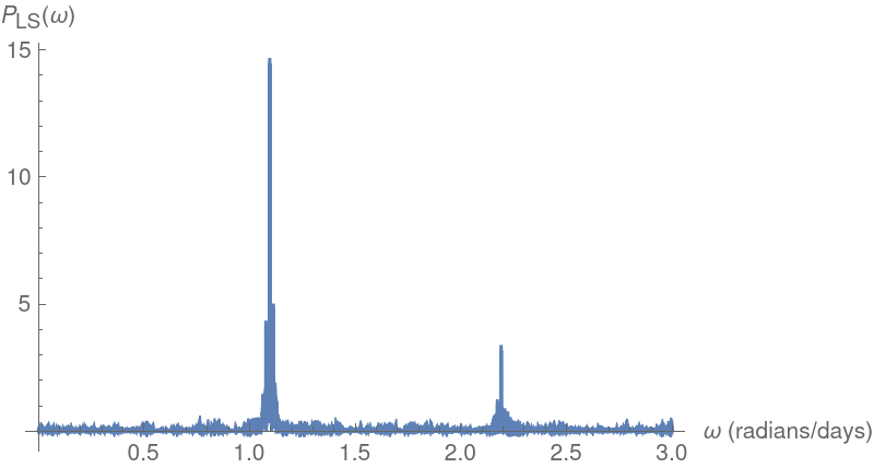
Plot the Lomb-Scargle periodogram and compute the corresponding estimated period:
Plot the Lafler-Kinman folded epoch total string lengths and compute the corresponding estimated period:
The period estimates all agree to several places. Plot the time series folded by epoch using the second one:
Searching for periodicity in a chromosome (12)
Coding sections of genes are well known to exhibit a periodicity of three base pairs (bp). Often there are other periodicities. There is a method for finding them, using chromosome 12 from Saccharomyces cerevisiae (baker’s yeast) as an example:
Literature on the subject states that it has a periodicity in the 10–11 range when looking at tetramers of the form A*T*, where the star here denotes zero or more occurrences of the preceding nucleotide (some specific values reported are 10, 10.2, 10.4 and 10.5). Split the chromosome into segments of 1000 bp and locate positions of the 4-mers "AAAA", "AAAT", "AATT", "ATTT" and "TTTT":
While there are various ways to turn a gene sequence into a numerical sequence, here the irregular periodogram is instead employed on common gaps between the positions found:
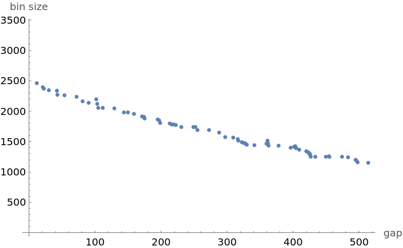
Smaller counts are discarded if there are more than 500. They are further decimated by removing all gap counts that are smaller than at least one of their 19 subsequent neighbors:
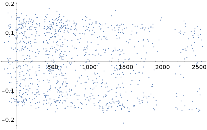
Plot the number of gaps as a function of gap size:
Treat gap lengths as the "time" variable and gap counts as the dependent variable:
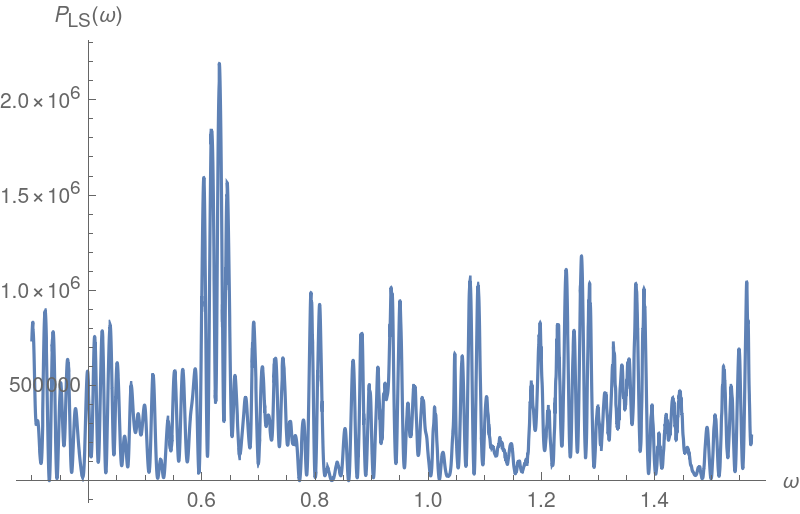
A periodicity of 3 is already known and larger ones are sought, so plot up to a frequency range that will only give periods of at least 4:
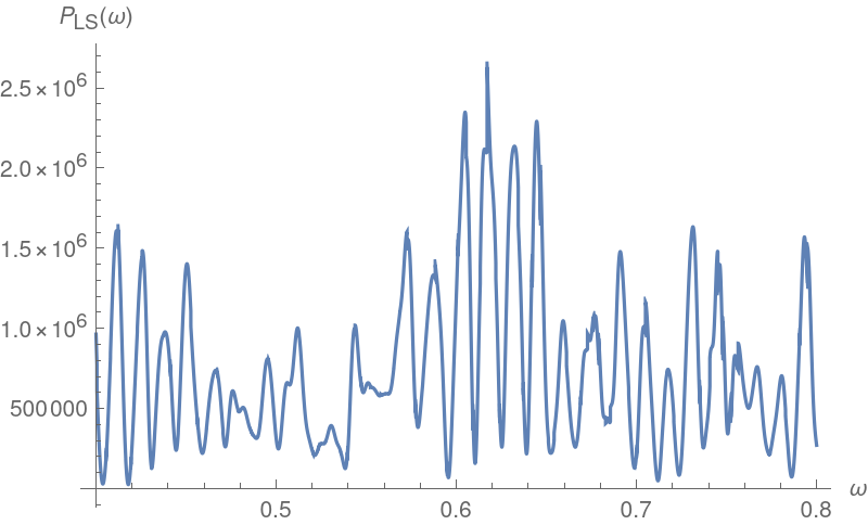
Isolate the large frequency near 0.6 to find a plausible periodicity value:
Homing in near 0.6 in the plot will show that there is a double peak, with the slightly larger one giving rise to a periodicity less than 10. This may be due to an interaction between the periodicity of 3 and the larger one. An attempt can be made to curtail this effect by repeating the periodogram computations on data that has had gaps that are multiples of 3 removed:
Home in near 0.6:
Recompute the period estimate:
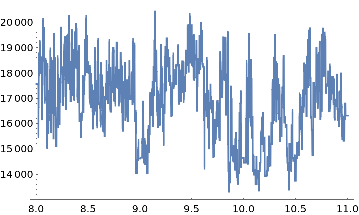
This is in line with values reported in the literature. A string-length plot and optimization gives a value in the same vicinity:
Different settings will give slightly different estimates; for example, with sublengths set to 5000 and upper set to 2000, the estimate is around 10.28. So the method here is viable but only to low precision.
Breaking a Vigenère cipher (15)
The Vigenère cipher is attacked from the Rosetta Code text example:
Split the text into trigrams and find the positions of each, retaining all that appear at least twice:
Find distances separating each given triad, and also retain the number of times a given distance appears (these lists will be used to assess the length of the key phrase):
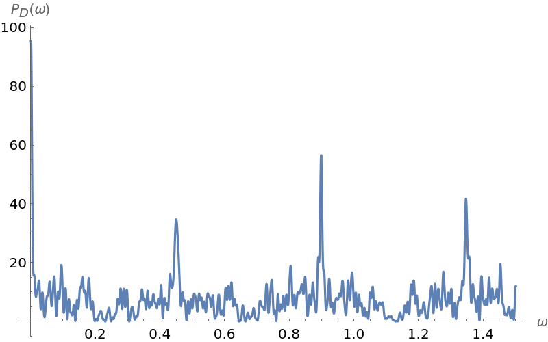
Use a periodogram to guess the length of the key phrase:
Find the period corresponding to the highest peak:
Find the period corresponding to the highest peak at lower frequency:
The key length guess of 14 is used because, in the worst-case scenario, it simply means a key phrase that is repeated is derived. First, list the most frequent letters in English in order of descending frequencies:
A "zero" value is also needed for character codes, so as to translate "A" to have the value 1:
A scoring heuristic is required to guess what the Caesar cipher shift is for each of the 14 letter subsets. It is based on numbers and positions of the most frequent letters in each subset that would, given a particular shift, map to letters that actually have the highest frequencies in English:
Code is also required to translate (decode) characters given a shift value:
Break the coded text into 14 distinct subsets; each will be treated as a Caesar cipher encoding. Find the most commonly appearing letters in each subset in order of descending frequency:
Find the top-scoring shift translation for each of the 14 cases:
Compute the corresponding shifts:
Use the shifts found to translate the key (this is not actually necessary for translating the encoded message):
Translate the encoded message:
![times = data[[All, 1]];
vals = data[[All, 2]] - Mean[data[[All, 2]]];
ListPlot[Transpose[{times, vals}]]](https://www.wolframcloud.com/obj/resourcesystem/images/320/3206d9de-59c6-4867-beea-bcc91a44f5e4/33e15dc60c295a17.png)
![Plot[ResourceFunction["IrregularPeriodogram"][w, times, vals], {w, .1,
5}, PlotPoints -> 300, PlotRange -> All, AxesLabel -> {"\[Omega] (radians)", "\!\(\*SubscriptBox[\(P\), \(D\)]\)(\[Omega])"}, ImageSize -> 400]](https://www.wolframcloud.com/obj/resourcesystem/images/320/3206d9de-59c6-4867-beea-bcc91a44f5e4/2c61f01c323a2147.png)
![Plot[ResourceFunction["IrregularPeriodogram"][p, times, vals, Method -> "LaflerKinman"], {p, 1, 8}, PlotPoints -> 300, PlotRange -> All, AxesLabel -> {"p", "\!\(\*SubscriptBox[\(P\), \(LK\)]\)(p)"}, ImageSize -> 400]](https://www.wolframcloud.com/obj/resourcesystem/images/320/3206d9de-59c6-4867-beea-bcc91a44f5e4/20e6c7bd9b1b3cd6.png)
![SeedRandom[11222333344444]
data2 = Sort[RandomSample[data, 20]];
times2 = data2[[All, 1]];
vals2 = data2[[All, 2]] - Mean[data2[[All, 2]]];
ListPlot[Transpose[{times2, vals2}]]](https://www.wolframcloud.com/obj/resourcesystem/images/320/3206d9de-59c6-4867-beea-bcc91a44f5e4/284400d265a481b7.png)
![Plot[ResourceFunction["IrregularPeriodogram"][w, times2, vals2], {w, .1, 5}, PlotPoints -> 300, PlotRange -> All, AxesLabel -> {"\[Omega] (radians)", "\!\(\*SubscriptBox[\(P\), \(D\)]\)(\[Omega])"}, ImageSize -> 400]](https://www.wolframcloud.com/obj/resourcesystem/images/320/3206d9de-59c6-4867-beea-bcc91a44f5e4/350559d41fb2d1bc.png)
![times = data[[All, 1]];
vals = data[[All, 2]] - Mean[data[[All, 2]]];
ListPlot[Transpose[{times, vals}]]](https://www.wolframcloud.com/obj/resourcesystem/images/320/3206d9de-59c6-4867-beea-bcc91a44f5e4/55b18e789028b407.png)
![Plot[ResourceFunction["IrregularPeriodogram"][w, times, vals], {w, .1,
5}, PlotPoints -> 300, PlotRange -> All, AxesLabel -> {"\[Omega] (radians/days)", "\!\(\*SubscriptBox[\(P\), \(D\)]\)(\[Omega])"}, ImageSize -> 400]](https://www.wolframcloud.com/obj/resourcesystem/images/320/3206d9de-59c6-4867-beea-bcc91a44f5e4/17678de28bb0bc9f.png)
![Plot[ResourceFunction["IrregularPeriodogram"][w, times, vals, Method -> "LombScargle"], {w, .1, 5}, PlotPoints -> 300, PlotRange -> All, AxesLabel -> {"\[Omega] (radians/days)", "\!\(\*SubscriptBox[\(P\), \(LS\)]\)(\[Omega])"}, ImageSize -> 400]](https://www.wolframcloud.com/obj/resourcesystem/images/320/3206d9de-59c6-4867-beea-bcc91a44f5e4/5ee1d4aea3ead204.png)
![freqLS = NArgMax[{ResourceFunction["IrregularPeriodogram"][w, times, vals, Method -> "LombScargle"], 2.5 <= w <= 3}, w];
perLS = 2 Pi/freqLS;
{freqLS, perLS}](https://www.wolframcloud.com/obj/resourcesystem/images/320/3206d9de-59c6-4867-beea-bcc91a44f5e4/72528430862ee23c.png)
![Plot[ResourceFunction["IrregularPeriodogram"][p, times, vals, Method -> "LaflerKinman"], {p, .1, 5}, PlotPoints -> 300, PlotRange -> All, AxesLabel -> {"p (days)", "\!\(\*SubscriptBox[\(L\), \(LK\)]\)(p)"}, ImageSize -> 400]](https://www.wolframcloud.com/obj/resourcesystem/images/320/3206d9de-59c6-4867-beea-bcc91a44f5e4/32ac22c6086fc161.png)
![perLK = NArgMin[{ResourceFunction["IrregularPeriodogram"][p, times, vals, Method -> "LaflerKinman"], 2. <= p <= 2.5}, p]](https://www.wolframcloud.com/obj/resourcesystem/images/320/3206d9de-59c6-4867-beea-bcc91a44f5e4/3d5075caaef632dd.png)
![SeedRandom[11222333344444]
data = Sort[
Map[{#, Sin[#] - 2*Sin[E*#] Cos[Sqrt[2]*#] + Cos[Pi*#]/2} &, RandomReal[{0, 20}, 800]]];
times = data[[All, 1]];
vals = data[[All, 2]] - Mean[data[[All, 2]]];
ListPlot[Transpose[{times, vals}]]](https://www.wolframcloud.com/obj/resourcesystem/images/320/3206d9de-59c6-4867-beea-bcc91a44f5e4/18657e73cc48c101.png)
![Plot[ResourceFunction["IrregularPeriodogram"][w, times, vals], {w, .1,
5}, PlotPoints -> 300, PlotRange -> All, AxesLabel -> {"\[Omega] (radians)", "\!\(\*SubscriptBox[\(P\), \(D\)]\)(\[Omega])"}, ImageSize -> 400]](https://www.wolframcloud.com/obj/resourcesystem/images/320/3206d9de-59c6-4867-beea-bcc91a44f5e4/0bab66029a75721c.png)
![SeedRandom[11222333344444]
data = Sort[
Map[{#, Sin[#] - 2*Sin[E*#] Cos[Sqrt[2]*#] + Cos[Pi*#]/2} &, RandomReal[{0, 20}, 20]]];
times = data[[All, 1]];
vals = data[[All, 2]] - Mean[data[[All, 2]]];
ListPlot[Transpose[{times, vals}]]](https://www.wolframcloud.com/obj/resourcesystem/images/320/3206d9de-59c6-4867-beea-bcc91a44f5e4/694e4dde06c8ecd3.png)
![Plot[ResourceFunction["IrregularPeriodogram"][w, times, vals], {w, .1,
5}, PlotPoints -> 300, PlotRange -> All, AxesLabel -> {"\[Omega] (radians)", "\!\(\*SubscriptBox[\(P\), \(D\)]\)(\[Omega])"}, ImageSize -> 400]](https://www.wolframcloud.com/obj/resourcesystem/images/320/3206d9de-59c6-4867-beea-bcc91a44f5e4/2058d95780d0ba10.png)
![SeedRandom[11222333344444]
times = Range[2, 20, .1];
data = Table[Sin[j] + Cos[3*j]/2 + .01*RandomReal[], {j, times}];](https://www.wolframcloud.com/obj/resourcesystem/images/320/3206d9de-59c6-4867-beea-bcc91a44f5e4/3066dfff34981579.png)
![Plot[ResourceFunction["IrregularPeriodogram"][w, times, vals], {w, .1,
5}, PlotPoints -> 300, PlotRange -> All, AxesLabel -> {"\[Omega] (radians)", "\!\(\*SubscriptBox[\(P\), \(D\)]\)(\[Omega])"}, ImageSize -> 400]](https://www.wolframcloud.com/obj/resourcesystem/images/320/3206d9de-59c6-4867-beea-bcc91a44f5e4/13b30153bcb43088.png)


![SeedRandom[11222333344444]
data = Sort[Map[{#, Sin[#] + Cos[3*#]/2} &, RandomReal[{0, 20}, 500]]];
times = data[[All, 1]];
vals = data[[All, 2]] - Mean[data[[All, 2]]];
Plot[irregPG[w, times, vals], {w, .1, 5}, PlotPoints -> 300, PlotRange -> All, AxesLabel -> {"\[Omega] (radians)", "\!\(\*SubscriptBox[\(P\), \(D\)]\)(\[Omega])"}]](https://www.wolframcloud.com/obj/resourcesystem/images/320/3206d9de-59c6-4867-beea-bcc91a44f5e4/17e67f6f2036d62a.png)
![tvpairs = monthsunspots["Path"];
tlist = tvpairs[[All, 1]];
vals = tvpairs[[All, 2]] - Mean[tvpairs[[All, 2]]];
times = N[(tlist - First[tlist])/(tlist[[2]] - First[tlist])];](https://www.wolframcloud.com/obj/resourcesystem/images/320/3206d9de-59c6-4867-beea-bcc91a44f5e4/6aa39eb3a737009b.png)
![Plot[ResourceFunction["IrregularPeriodogram"][w, times, vals, Method -> "Deeming"], {w, .001, .1}, PlotPoints -> 300, PlotRange -> All, AxesLabel -> {"\[Omega] (radians/months)", "\!\(\*SubscriptBox[\(P\), \(LS\)]\)(\[Omega])"}, ImageSize -> 400]](https://www.wolframcloud.com/obj/resourcesystem/images/320/3206d9de-59c6-4867-beea-bcc91a44f5e4/62465081f91f2080.png)
![freqD = NArgMax[{ResourceFunction["IrregularPeriodogram"][w, times, vals, Method -> "Deeming"], .045 <= w <= .06}, w];
perD = 2*Pi/freqD;
{freqD, perD}](https://www.wolframcloud.com/obj/resourcesystem/images/320/3206d9de-59c6-4867-beea-bcc91a44f5e4/177343b2c974a112.png)
![Plot[ResourceFunction["IrregularPeriodogram"][w, times, vals, Method -> "LombScargle"], {w, .001, .1}, PlotPoints -> 300, PlotRange -> All, AxesLabel -> {"\[Omega] (radians/months)", "\!\(\*SubscriptBox[\(P\), \(LS\)]\)(\[Omega])"}, ImageSize -> 400]](https://www.wolframcloud.com/obj/resourcesystem/images/320/3206d9de-59c6-4867-beea-bcc91a44f5e4/6d10f14aa0141ece.png)
![freqLS = NArgMax[{ResourceFunction["IrregularPeriodogram"][w, times, vals, Method -> "LombScargle"], .04 <= w <= .06}, w];
perLS = 2*Pi/freqLS;
{freqLS, perLS}](https://www.wolframcloud.com/obj/resourcesystem/images/320/3206d9de-59c6-4867-beea-bcc91a44f5e4/71762be128ace9e2.png)
![ListPlot[lkvals = Table[ResourceFunction["IrregularPeriodogram"][p, times, vals, Method -> "LaflerKinman"], {p, 1, 300, .1}]]](https://www.wolframcloud.com/obj/resourcesystem/images/320/3206d9de-59c6-4867-beea-bcc91a44f5e4/632d5eee67056c1a.png)
![GraphicsRow[{ListPlot[Transpose[{foldTimes[times, perLS], vals}]], ListPlot[Transpose[{foldTimes[times, perLK], vals}]], ListPlot[Transpose[{foldTimes[times, 12*11], vals}]]}]](https://www.wolframcloud.com/obj/resourcesystem/images/320/3206d9de-59c6-4867-beea-bcc91a44f5e4/56a83b2e472cdbdc.png)
![cep2308Idata = Import["http://ogledb.astrouw.edu.pl/~ogle/CVS/data/I/08/OGLE-LMC-CEP-2308.dat", "Table"][[All, 1 ;; 2]]; {times2308, ovalues2308} = Transpose[cep2308Idata]; times2308 = times2308 - times2308[[1]]; mean2308 = Mean[ovalues2308]; values2308 = ovalues2308 - mean2308;](https://www.wolframcloud.com/obj/resourcesystem/images/320/3206d9de-59c6-4867-beea-bcc91a44f5e4/248a3fe42dfe8a40.png)
![Plot[ResourceFunction["IrregularPeriodogram"][w, times2308, values2308, Method -> "Deeming"], {w, .001, 3}, PlotPoints -> 300, PlotRange -> All, AxesLabel -> {"\[Omega] (radians/days)", "\!\(\*SubscriptBox[\(P\), \(D\)]\)(\[Omega])"}, ImageSize -> 400]](https://www.wolframcloud.com/obj/resourcesystem/images/320/3206d9de-59c6-4867-beea-bcc91a44f5e4/55df8e7420eef345.png)
![freqD = NArgMax[{ResourceFunction["IrregularPeriodogram"][w, times2308, values2308], .8 <= w <= 1.3}, w];
perD = 2 Pi/freqD;
{freqD, perD}](https://www.wolframcloud.com/obj/resourcesystem/images/320/3206d9de-59c6-4867-beea-bcc91a44f5e4/348dbfedac15cd05.png)
![Plot[ResourceFunction["IrregularPeriodogram"][w, times2308, values2308, Method -> "LombScargle"], {w, .001, 3}, PlotPoints -> 300, PlotRange -> All, AxesLabel -> {"\[Omega] (radians/days)", "\!\(\*SubscriptBox[\(P\), \(LS\)]\)(\[Omega])"}, ImageSize -> 400]](https://www.wolframcloud.com/obj/resourcesystem/images/320/3206d9de-59c6-4867-beea-bcc91a44f5e4/5e3d4d1a97776dca.png)
![freqLS = NArgMax[{ResourceFunction["IrregularPeriodogram"][w, times2308, values2308, Method -> "LombScargle"], .8 <= w <= 1.3},
w];
perLS = 2 Pi/freqLS;
{freqLS, perLS}](https://www.wolframcloud.com/obj/resourcesystem/images/320/3206d9de-59c6-4867-beea-bcc91a44f5e4/7df4a58ee878ae60.png)
![Plot[ResourceFunction["IrregularPeriodogram"][w, times2308, values2308, Method -> "LaflerKinman"], {w, .001, 20}, PlotPoints -> 300, PlotRange -> All, AxesLabel -> {"\[Omega] (radians/months)", "\!\(\*SubscriptBox[\(P\), \(LS\)]\)(\[Omega])"}, ImageSize -> 400]](https://www.wolframcloud.com/obj/resourcesystem/images/320/3206d9de-59c6-4867-beea-bcc91a44f5e4/5d4836f4af40d61a.png)
![perLK = NArgMin[{ResourceFunction["IrregularPeriodogram"][p, times2308, values2308, Method -> "LaflerKinman"], 5.4 <= p <= 6}, p]](https://www.wolframcloud.com/obj/resourcesystem/images/320/3206d9de-59c6-4867-beea-bcc91a44f5e4/63c1960637f0b0b7.png)
![seq = Import[
"ftp://ftp.ensembl.org/pub/release-81/fasta/saccharomyces_cerevisiae/dna/Saccharomyces_cerevisiae.R64-1-1.dna_rm.chromosome.XII.fa.gz"];
chromo = seq[[1]];](https://www.wolframcloud.com/obj/resourcesystem/images/320/3206d9de-59c6-4867-beea-bcc91a44f5e4/284068f96a9d1598.png)
![chromos = StringSplit[chromo, "N"] /. "" :> Nothing;
sublengths = 1000;
subchromos = Flatten[Map[StringPartition[#, sublengths] &, chromos]];
at4 = "AAAA" | "AAAT" | "AATT" | "ATTT" | "TTTT";
posnlists = Map[StringPosition[#, at4][[All, 1]] &, subchromos];](https://www.wolframcloud.com/obj/resourcesystem/images/320/3206d9de-59c6-4867-beea-bcc91a44f5e4/5c48fcf26ce66636.png)
![pdiffs = Flatten[
Table[Outer[Subtract, posnsj, posnsj], {posnsj, posnlists}]];
pdiffs = DeleteCases[pdiffs, aa_ /; aa <= 0];
tallies = Tally[pdiffs];
talliesS = Sort[tallies];](https://www.wolframcloud.com/obj/resourcesystem/images/320/3206d9de-59c6-4867-beea-bcc91a44f5e4/71a622241517fff6.png)
![grouped = Partition[talliesS, 20, 1];
upper = 500;
groupedS = DeleteDuplicates[
Map[First[SortBy[#, -#[[2]] &]] &, grouped[[2 ;; UpTo[upper]]]]];](https://www.wolframcloud.com/obj/resourcesystem/images/320/3206d9de-59c6-4867-beea-bcc91a44f5e4/7306d9a196ffe1d0.png)
![Plot[ResourceFunction["IrregularPeriodogram"][w, timesC, valsC, Method -> "LombScargle"], {w, .3, 2*Pi/4}, PlotPoints -> 500, PlotRange -> All, AxesLabel -> {"\[Omega]", "\!\(\*SubscriptBox[\(P\), \(LS\)]\)(\[Omega])"}, ImageSize -> 400]](https://www.wolframcloud.com/obj/resourcesystem/images/320/3206d9de-59c6-4867-beea-bcc91a44f5e4/668709df441c83be.png)
![freqLS = NArgMax[{ResourceFunction["IrregularPeriodogram"][w, timesC, valsC, Method -> "LombScargle"], .5 <= w <= .7}, w];
perLS = 2*Pi/freqLS;
{freqLS, perLS}](https://www.wolframcloud.com/obj/resourcesystem/images/320/3206d9de-59c6-4867-beea-bcc91a44f5e4/3a6382eb87b03621.png)
![{timesC, valsC} = Transpose[Select[groupedS, (! IntegerQ[#[[1]]/3]) &]];
valsC = valsC - Mean[N@valsC];
Plot[ResourceFunction["IrregularPeriodogram"][w, timesC, valsC, Method -> "LombScargle"], {w, .3, 2*Pi/4}, PlotPoints -> 500, PlotRange -> All, AxesLabel -> {"\[Omega]", "\!\(\*SubscriptBox[\(P\), \(LS\)]\)(\[Omega])"}, ImageSize -> 400]](https://www.wolframcloud.com/obj/resourcesystem/images/320/3206d9de-59c6-4867-beea-bcc91a44f5e4/392eb48852bcc1ad.png)
![Plot[ResourceFunction["IrregularPeriodogram"][w, timesC, valsC, Method -> "LombScargle"], {w, .4, .8}, PlotPoints -> 500, PlotRange -> All, AxesLabel -> {"\[Omega]", "\!\(\*SubscriptBox[\(P\), \(LS\)]\)(\[Omega])"}, ImageSize -> 400]](https://www.wolframcloud.com/obj/resourcesystem/images/320/3206d9de-59c6-4867-beea-bcc91a44f5e4/1b50ad02ac42cb4e.png)
![freqLS = NArgMax[{ResourceFunction["IrregularPeriodogram"][w, timesC, valsC, Method -> "LombScargle"], .4 <= w <= .8}, w];
perLS = 2*Pi/freqLS;
{freqLS, perLS}](https://www.wolframcloud.com/obj/resourcesystem/images/320/3206d9de-59c6-4867-beea-bcc91a44f5e4/600d422695983e43.png)
![Plot[ResourceFunction["IrregularPeriodogram"][p, timesC, valsC, Method -> "LaflerKinman"], {p, 8, 11}, PlotRange -> All]](https://www.wolframcloud.com/obj/resourcesystem/images/320/3206d9de-59c6-4867-beea-bcc91a44f5e4/24b28541493af576.png)
![text = StringDelete[
"MOMUD EKAPV TQEFM OEVHP AJMII CDCTI FGYAG JSPXY ALUYM NSMYH
VUXJE LEPXJ FXGCM JHKDZ RYICU HYPUS PGIGM OIYHF WHTCQ KMLRD
ITLXZ LJFVQ GHOLW CUHLO MDSOE KTALU VYLNZ RFGBX PHVGA LWQIS
FGRPH JOOFW GUBYI LAPLA LCAFA AMKLG CETDW VOELJ IKGJB XPHVG
ALWQC SNWBU BYHCU HKOCE XJEYK BQKVY KIIEH GRLGH XEOLW AWFOJ
ILOVV RHPKD WIHKN ATUHN VRYAQ DIVHX FHRZV QWMWV LGSHN NLVZS
JLAKI FHXUF XJLXM TBLQV RXXHR FZXGV LRAJI EXPRV OSMNP KEPDT
LPRWM JAZPK LQUZA ALGZX GVLKL GJTUI ITDSU REZXJ ERXZS HMPST
MTEOE PAPJH SMFNB YVQUZ AALGA YDNMP AQOWT UHDBV TSMUE UIMVH
QGVRW AEFSP EMPVE PKXZY WLKJA GWALT VYYOB YIXOK IHPDS EVLEV
RVSGB JOGYW FHKBL GLXYA MVKIS KIEHY IMAPX UOISK PVAGN MZHPW
TTZPV XFCCD TUHJH WLAPF YULTB UXJLN SIJVV YOVDJ SOLXG TGRVO
SFRII CTMKO JFCQF KTINQ BWVHG TENLH HOGCS PSFPV GJOKM SIFPR
ZPAAS ATPTZ FTPPD PORRF TAXZP KALQA WMIUD BWNCT LEFKO ZQDLX
BUXJL ASIMR PNMBF ZCYLV WAPVF QRHZV ZGZEF KBYIO OFXYE VOWGB
BXVCB XBAWG LQKCM ICRRX MACUO IKHQU AJEGL OIJHH XPVZW JEWBA
FWAML ZZRXJ EKAHV FASMU LVVUT TGK", Whitespace];](https://www.wolframcloud.com/obj/resourcesystem/images/320/3206d9de-59c6-4867-beea-bcc91a44f5e4/5574c640e1aa000f.png)
![triads = StringPartition[text, 3, 1];
unique = Union[triads];
mposns = Map[Flatten, DeleteCases[Map[Position[triads, #] &, unique], aa_ /; Length[aa] < 2]]](https://www.wolframcloud.com/obj/resourcesystem/images/320/3206d9de-59c6-4867-beea-bcc91a44f5e4/0262acd21d67f735.png)


![Plot[ResourceFunction["IrregularPeriodogram"][w, permults, lens], {w, 0, 1.5}, PlotPoints -> 400, PlotRange -> All,
AxesLabel -> {"\[Omega]", "\!\(\*SubscriptBox[\(P\), \(D\)]\)(\[Omega])"}, ImageSize -> 400]](https://www.wolframcloud.com/obj/resourcesystem/images/320/3206d9de-59c6-4867-beea-bcc91a44f5e4/6378ad2ddd00a4e1.png)
![score[startchar_, l1_, letters_] := Module[
{diff = startchar - ToCharacterCode[l1][[1]], newletters, s1, s2, badposns},
newletters = anumminus + Mod[Flatten[ToCharacterCode[letters]] - anumminus + diff, 26, 1];
s2 = Map[Position[Complement[topchars, {startchar}], #] &, newletters];
s1 = Range[Length[s2]] . Flatten[(s2 /. {} -> 0)];
badposns = Flatten[Position[s2, {}]];
10*Total[15 - badposns] + s1
]
scores[l1_, letters_] := Map[score[#, l1, letters] &, topchars]](https://www.wolframcloud.com/obj/resourcesystem/images/320/3206d9de-59c6-4867-beea-bcc91a44f5e4/2add8495cd514674.png)
![diff[{posn_, letter_}] := ToCharacterCode[letter][[1]] - topchars[[posn]]
translate[nums_, diff_] := FromCharacterCode[anumminus + Mod[nums - diff - anumminus, 26, 1]]](https://www.wolframcloud.com/obj/resourcesystem/images/320/3206d9de-59c6-4867-beea-bcc91a44f5e4/02116e7bc40e2167.png)
![caesars = Transpose[Partition[Characters[text], 14]];
caesarnums = Map[ToCharacterCode[#] &, caesars];
tops = Map[Take[ReverseSortBy[Tally[#], Last], 8][[All, 1]] &, caesars]](https://www.wolframcloud.com/obj/resourcesystem/images/320/3206d9de-59c6-4867-beea-bcc91a44f5e4/7879bc7e55be3fa6.png)